Ilhan Aydin* | Seyfullah Kaner
© 2020 IIETA. This article is published by IIETA and is licensed under the CC BY 4.0 license (http://creativecommons.org/licenses/by/4.0/).
OPEN ACCESS
Induction motors are an essential component of many applications in industry due to their robust and simple construction. Since bearing faults are the most occurred fault type in the induction motors, it is important to implement the fault detection procedure at an early stage to prevent a sudden interruption of industrial systems. In recent years, deep learning-based techniques have become important tools for converting raw data into images and for producing high-quality images. However, deep learning-based techniques are still difficult to apply in real-time because the techniques require large training data, which slows down the learning process. In the present study, we propose a novel bearing faults diagnosis method at different operating speeds and load conditions. We obtain the time-frequency (TF) representation by applying continuous wavelet analysis to the raw vibration signals. The results of TF representation is recorded as an image. We apply co-occurrence Histograms of Oriented Gradients (coHOG) to the image to obtain features and classify the features with extreme learning machine with a sparse classifier (ELMSRC) to diagnose faults. We obtained better results in terms of time and performance compared with the proposed method of other classification and deep learning techniques.
bearing faults, classification, extreme learning machine with sparse classifier, fault diagnosis, feature extraction, time-frequency images
Induction motors are essential components of manufacturing systems and account for 80% of the workforce in the industry [1]. However, long-term operation and exposure to moisture and dust in the working environment may provoke faults [2], which may consequently affect the system reliability. Bearing faults are the most common type of mechanical faults that occurs in induction motors. Early and accurate diagnosis of these faults has been a main requirement of many industrial systems [3, 4].
Generally, fault diagnosis methods are classified into three categories: mathematical model, processing of some signals, and intelligent methods [5]. Mathematical model-based methods detect faults according to the change of certain parameters in the model. Intelligent fault diagnosis methods are to collect substantial amounts of data to represent each fault condition accurately [6]. This method is useful for complex systems, especially where it is difficult to construct a precise model. In recent years, big data can be acquired from any system faster with the development of intelligent manufacturing and industry 4.0 [7]. The performance of intelligent diagnostic methods for training depends on the amount of data; however, this is unsuitable for the detection of the unknown conditions [8]. In complex diagnostics problems, signal processing techniques such as fast Fourier transform and wavelet analysis are used to extract features from a signal [9].
Although signals such as current and temperature are also used to detect bearing faults, these faults give better symptoms on vibration signals. The sequential and periodic oscillations occurred when the bearing component passes through the defective point. These oscillations appear as a pattern in vibration signals. Time and frequency analysis of vibration signals were performed to determine ball, inner, and outer ring faults [10-14]. Multiple domain features were obtained from vibration signals and the faults occurred on rotating machinery were detected [15]. Fast Fourier Transform is the most fundamental frequency-based method to detect bearing faults [16, 17]. However, in the spectrum obtained by the Fourier transform, the frequencies associated with bearing faults are difficult to distinguish because of noise. To overcome the problems related to the Fast Fourier transform, short time Fourier transform (STFT) [18], wavelet and Gabor analysis [19, 20], Hilbert transform [21], park vector transformation [22], and phase space reconstruction [23] were proposed to detect bearing related faults. In contrast with the Fourier transform, wavelet analysis inspects the signal in the TF domain, effective in detecting inner and outer race faults using non-stationary signals. Envelope analysis-based techniques have been proposed to improve the fault diagnosis performance of frequency-based methods [24]. The envelope spectrum is more distinctive compared to the original signal spectrum. Using specific preprocessing methods or statistical properties from raw data, time domain-based methods are used to detect bearing faults signals. An intelligent filter-based method for detecting bearing faults is presented [13]. Their method learns healthy condition with the aid of the Adaline filtering technique. Although the method offers good results in inner and outer race faults, it obtains low performance in ball faults. The features obtained in TF domain were given to an Adaptive Neuro-fuzzy Inference System (ANFIS) system, and bearing faults were diagnosed [12]. In recent years, the development of deep learning methods has facilitated the applications of the fault diagnosis. The motor bearing condition was detected by feeding raw vibration signals to a one-dimensional Convolutional Neural Network (CNN) [25]. Vibration signal was converted to a two-dimensional matrix, and a gray image was obtained and trained with deep learning algorithm in order to classify bearing faults [26]. However, this method provides no detailed information about the frequency of the fault as the signal changes over time.
In this study, a new method based on TF representation, coHOG and sparse classifier is proposed for the diagnosis of bearing faults. The features were obtained by applying coHOG transform to TF image obtained by continuous wavelet analysis. Since the coHOG method represents an image with multiple gradient orientations, it obtains more detailed features in the image than HOG method. A sparse classifier based on extreme learning machine is proposed and the related features are selected to improve the classification performance. This study provides the following main contributions:
The rest of the paper is organized as follows: Section 2 discusses the bearing fault diagnosis problem. Section 3 presents the proposed fault diagnosis method, preprocessing of the raw vibration signal via TF image, and overview of the feature extraction and classification. In section 4, the efficiency of our method is verified using an experimental data. Section 5 presents the conclusions.
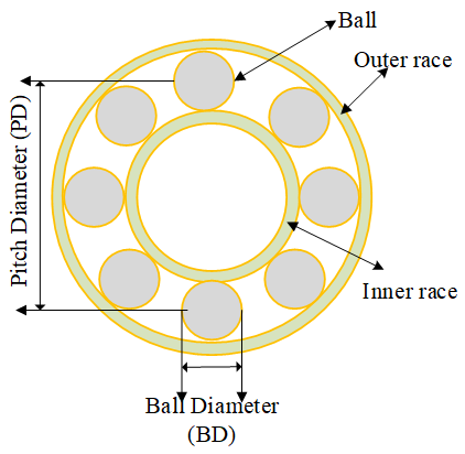
Bearing components are the most commonly used elements in electrical machinery, and these may provoke a fault that may lead to a machine breakdown. Bearing faults generally occur in the inner race, the outer race, and the rolling ball [27]. The vibration signal is the most commonly used signal for the bearing faults detection because of a change in the fault. For example, when outer race fault occurs, a peek is formed at certain intervals, which disturbs the vibration signal. The geometry of a ball bearing is shown in Figure 1.
Figure 1. Bearing geometry
In Figure 1, the fault in each component causes changes in frequency components and frequency spectrum. To calculate the location of the frequency components, parameters such as shaft speed, ball diameter, and pitch diameter should be known. The spectral frequencies for each fault type are calculated as follows:
$B P F O=\frac{n f_{r}}{2}\left(1-\frac{B D}{P D} \cos \phi\right)$ (1)
where, fr represents the shaft speed in revolutions per second, and n is the number of balls. BD and PD parameters indicate the ball diameter pitch diameter, respectively. The angle φ represents the contact angle, and this parameter is taken as zero for ball bearings.
$B P F I=\frac{n f_{r}}{2}\left(1+\frac{B D}{P D} \cos \phi\right)$ (2)
$B S F=\frac{P D}{2 B D}\left[1-\left(\frac{B D}{P D} \cos \phi\right)^{2}\right]$ (3)
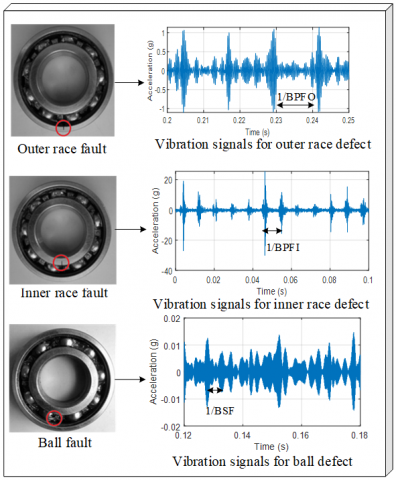
The effects of each fault on the vibration signal are different from each other, and the condition of the components in the bearing is determined by analyzing different frequency components. Figure 2 shows the representation of the vibration signals according to the faults.
Figure 2. Typical vibration signals from each fault of the rolling element bearing
Figure 2 reveals an oscillation at specific frequencies for each fault type, used to obtain frequency information related to the fault. The main issue is to find the oscillation peak and determine the frequency of the fault. For this purpose, the envelope analysis is the most known method. Figure 3 shows the frequencies related to the inner race fault in the frequency spectrum.
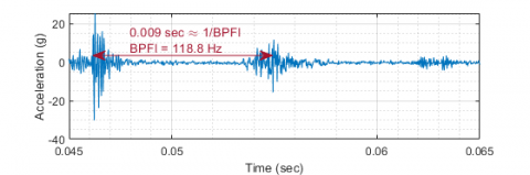
(a) Calculation of the BPFI frequency
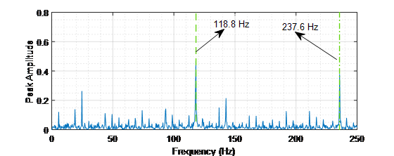
(b) Frequency spectrum of the signal and BPFI frequencies
Figure 3. Demonstration of BPFI calculation and frequency spectrum for inner race fault
When examining the signal in the time domain in Figure 3 (a), the amplitude of the original signal is modulated at a certain frequency. This frequency is set to 118.8 Hz by dividing the time between oscillations. In Figure 3 (b), frequencies related to inner race fault are shown in the frequency spectrum. Although envelope analysis is used to obtain the fault-related frequencies, certain parameters must be adjusted to determine peaks signal. The equations to estimate frequency requires knowledge of the ball and pitch diameters, shaft speed, number of balls, and contact angle. However, an additional speed sensor is required to measure the shaft speed.
A new hybrid method is proposed for the diagnosis of bearing faults, which uses TF representation, coHOG, and extreme learning-based sparse classifiers. The TF representation for the different fault types and the healthy condition provides a distinctive representation. Features are extracted from the images obtained with the help of coHOG, and faults are classified using a sparse classifier. The block diagram of the proposed method is given in Figure 4.
In Figure 4, vibration signals are transformed into a time-frequency domain using a continuous wavelet transform. Afterwards, the obtained time-frequency domain matrix is converted to an 8-bit grayscale image. The texture features are obtained from this image using coHOG, which extracts the shape of the image and the features using gradient orientations with different offsets. The features obtained from coHOG represent a sparse structure. Therefore, a sparse classifier is applied to these features to classify faults. Extreme Learning Machine (ELM) based sparse classifier is proposed to separate features and classify each condition [28]. The detail of each step of the proposed method is discussed in the following subsections.
Figure 4. The block diagram of the proposed method
3.1 Time-frequency representation
A TF analysis of the signal obtained from the vibration sensor was performed to obtain the TF image. Typically, TF image analysis is the technique that assists in studying a time series in the time-frequency domain. This technique helps a signal to display frequency information over time and produces different patterns for different operating conditions. Techniques such as short-time Fourier transform [29] s-transform [30, 31], Wigner-Ville distribution [32], and continuous-time wavelet [33, 34] are used to obtain TF representation. Continuous wavelet analysis is more effective as it represents the signal with multiple resolutions compared with other methods [35, 36]. Continuous wavelet analysis was used to determine the winding faults in the current signals of the steady-state and to extract the features to determine bearing faults from vibration signals [37].
Wavelet analysis uses a signal and a wavelet function, based on their inner products and the similarity between them. The analysis function is in continuous wavelet analysis used to compare the signal with shifted and scaled versions of a wavelet function [38]. A 2-dimensional representation is obtained by comparing the wavelet of different scales and positions. The set of wavelets is obtained by scaling and translating the mother wavelet as shown in (4).
$\psi_{a, b}(t)=\frac{1}{\sqrt{a}} \Psi\left(\frac{t-b}{a}\right)$ (4)
where,
is a scaling parameter, inversely proportional to frequency. The parameter b represents the translation. Continuous wavelet transform of a signal I(t) is given in (5).$W_{I}(b, a)=\frac{1}{\sqrt{a}} \int_{-\infty}^{\infty} I(t) \Psi^{*}\left(\frac{t-b}{a}\right) d t$ (5)
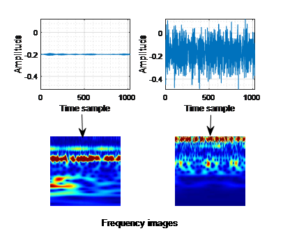
In (5), * represents the complex conjugate value of $\psi$ function. The coefficients of the continuous wavelet analysis affect the scaling, position values, and the used wavelets. Using scaled and shifted versions of the wavelet function [39], continuous wavelet analysis employs variable-sized windows to maintain time dependence. With the signal I(t), the wavelet coefficients of any scale $a$ are obtained using the convolution of the transformed and dilated versions of the wavelet. The higher coefficients represent the position of a particular event. After the convolution operator, the original signal I(t) is projected to 2D time and scale dimension, in which the scalogram represents the graphical representation of wavelet coefficients. For two different conditions, the signals and their TF images are given in Figure 5.
Figure 5. Healthy and faulty signals and their time-frequency images
In Figure 5, the left signal was acquired from a healthy motor; whereas, the right signal was acquired from a motor with ball bearing fault. When the TF images of both signals are examined, they are quite different. After obtaining time-frequency images, the features are extracted from the images using the coHOG method.
3.2 Feature extraction using coHOG
HOG transform, a popular tool for image classification [40], uses the orientation and magnitude values of the pixels in the image; which helps an independent descriptor of rotation. Moreover, HOG transform offers good results under different working conditions. The main goal of HOG is to define the image as a group of local histograms that produces the number of orientations within the respective region. To obtain HOG from an image, the color image is converted to a gray image. Afterward, the horizontal fx and vertical fy gradients are calculated using the derivative masks of the image. These gradients are calculated as follows.
$\begin{array}{l}
f_{x}(x, y)=I(x+1, y)-I(x-1, y), \forall x, y \\
f_{y}(x, y)=I(x, y+1)-I(x, y-1), \forall x, y
\end{array}$ (6)
In (6), I(x, y) represents the pixel density at the position of (x, y). The magnitude (m) and orientation $\theta$ are calculated as follows.
$m(x, y)=\sqrt{f_{x}(x, y)^{2}+f_{y}(x, y)^{2}}$ (7)
$\theta(x, y)=\tan ^{-1}\left(\frac{f_{y}(x, y)}{f_{x}(x, y)}\right)$ (8)
In the next step, the image is divided into cells of a certain size, and the orientations within each cell are assigned to eight bins. Then, the magnitudes of the orientations are voted for each bin. Histogram bins are constructed with equal sizes between 0-180 degrees.
After the orientation of each cell is obtained, block normalization is applied to the feature vector. For this purpose, L2-norm normalization is used, and its calculation is given in (9).
$f=\frac{v}{\sqrt{|v|^{2}+1}}$ (9)
Figure 6. The steps of coHOG transform
In (9), f and v represent the normalized and un-normalized histogram vector, respectively. HOG transform is used for real-time applications owing to its low-cost implementation. However, this method fails to offer the correct results in many object recognition problems since it shows the image with a single gradient orientation. Therefore, coHOG method, which shows the spatial relationship between gradient orientations, has been proposed [41]. This is a multi-gradient orientation based method represented as gradient pairs. Therefore, coHOG feature vector, built from pairs of gradient orientations, is better than HOG and the histogram. This vector is called a co-occurrence matrix. The coHOG feature is obtained from the 2D histogram of gradient orientation pairs in a given offset neighborhood. coHOG is applied to a gray image. Figure 6 shows the steps of the coHOG transformation to obtain the co-occurrence matrices.
In Figure 6, co-occurrence matrices are calculated for all offset values in each tiled region. All components of the obtained co-occurrence matrices are concatenated as a vector. After the horizontal and vertical gradients of the image are obtained with appropriate filters, the gradient orientations of the image are calculated. Afterwards, each pixel is labeled with one of eight different orientations with 45-degree angles in the range of (0,360). Combining the gradient orientations of neighbor offsets provides a detailed representation of the object. The offset (x, y) of a co-occurrence matrix over an N×M image is given in (10).
$C_{x, y}(i, j)=\sum_{t=1}^{N} \sum_{v=1}^{M}\left\{\begin{array}{ll}
1, & \text { If } I(t, v)=i \text { and } \\
& I(t+x, v+y)=j \\
0, & \text { otherwise }
\end{array}\right.$ (10)
In (10), I represent the gradient orientation image, whereas, i and j represent gradient orientations. The offset on horizontal and vertical orientations are given by x and y, respectively. For each motor condition, a feature vector is obtained by coHOG, and the obtained vector is given to the classifier and fault conditions.
3.3 Extreme learning machine and sparse representation based classifier
ELM is a classification method and its structure is a feedforward neural network with a single hidden layer [42]. The main difference between ELM and ANN is that ELM randomly generates the parameters in the hidden layer and learns the weights analytically rather than iterative learning as in the backpropagation algorithm.
The mathematical model of ELM, which has L nodes in the hidden layer and an activation function g(x), is as follows.
$\begin{array}{l}
o_{j}=\sum_{i=1}^{L} \beta_{i} g_{i}\left(w_{i} \cdot x_{j}+b_{i}\right) \\
j=1,2, \ldots, N
\end{array}$ (11)
In (11), xj and bi represent jth input and ith randomly chosen bias value, respectively. The parameter N represents the number of training samples, and L is a number of hidden nodes. The vectors wi=[wi1, wi2, …, win]T and βi=[Βi1, βi2, …, βim]T represent the weight vectors connecting input neurons to ith hidden neuron and ith hidden neuron to output neuron oj, respectively. The real output of ELM is ti=[ti1, t2i, …, tim]T. The aim of ELM is to minimize the relative error between real output ti and model output oj. The minimization equation is modeled as follows:
$H \beta=T$ (12)
In (12), H represents the output of the hidden layer, and the output matrix of the classifier is given by T. The two matrices are given in (13) and (14), respectively.
$H=\left[\begin{array}{ccc}
g\left(w_{1} \cdot x_{1}+b_{1}\right) & \cdots & g\left(w_{L} \cdot x_{1}+b_{L}\right) \\
\vdots & \cdots & \vdots \\
g\left(w_{1} \cdot x_{N}+b_{1}\right) & & g\left(w_{L} \cdot x_{N}+b_{L}\right)
\end{array}\right]$ (13)
$T=\left[\begin{array}{c}
t_{1}^{T} \\
\vdots \\
t_{N}^{T}
\end{array}\right]_{N X m}$ (14)
In (13), each column of H matrix is an output of a hidden node with respect to inputs. Each row of the T matrix represents the output of ELM with respect to an input. The optimal output weight matrix is given in (15).
$\bar{\beta}=H^{-1} T$ (15)
where, H-1 represent inverse of H. The ELM classifier can learn huge data and work quickly with parallel computing. The most important feature of ELM is that all parameters in the hidden layer are randomly generated, and the weights in the output layer are analytically solved without tuning, which shortens the test time. However, the ELM classifier gives incorrect results owing to the image noise. Moreover, high performance is not achieved during the training stage and testing stage. In the sparse representation classification (SRC), training sets are used to classify test data. This method offers good results, especially in facial recognition applications. Assuming we have a training image set with multiple classes, the main aim of the sparse classifier is to obtain a sparse representation of a test image in the training set. Suppose, we have a set of training data with class labels C = [c1, c2, c3...cm], to classify a test data y, the columns of C are normalized using l2-norm. The following optimization problem is solved as:
$\begin{array}{l}
\hat{x}=\arg \min _{x}\|A x-y\|_{2}^{2}+ \\
\lambda \sum_{i=1}^{D} x_{i}, x_{i}>0, i=1,2, \cdots, D
\end{array}$ (16)
In (16), D is the number of training images. Only the non-zero entries in x are associated with the class i, which is represented by the δi(x) vector. The class of the test image y is computed according to the minimum distance between y and Aδi(x). The related equation is given in (17).
$\text { Class }(y)=\operatorname{argmin}_{i}\left\{\left\|y-A \delta_{i}(\hat{x})\right\|_{2}\right\}$ (17)
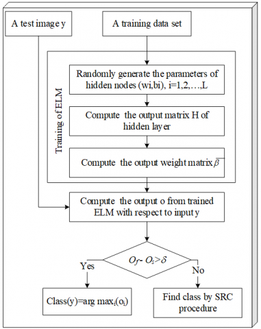
The SRC method uses all training images to determine the class of any test image, and direct use of SRC causes the classifier to run slowly. Therefore, the combination of ELM and SRC can make the SRC operate in case of noisy data that cause a false alarm. In other cases, the ELM should operate [28]. A combination of ELM and SRC is called ELMSRC, used to improve the classification performance. Figure 7 provides the steps of this method.
In Figure 7, the features obtained by coHOG are input into the ELM classifier and the ELM training parameters. The outputs are obtained by giving a test image y to a trained ELM classifier. For this test image, the difference between the first and second-largest output of the ELM classifier is compared with the threshold value to determine whether the image has noise or not. Images without any noise are classified according to the ELM rule, whereas images, smaller than the threshold value are classified with SRC.
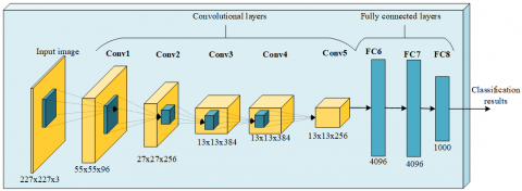
For comparison purposes, the images obtained by TF representation were also classified with a deep learning algorithm. For this purpose, Alexnet's deep convolutional neural network structure, proposed by Krizhevsky et al. [43] was used. Alexnet has 5 convolution layers, 11x11 filters and 3 fully connected layers. Alexnet is an important algorithm for image classification with a total of 60 million parameters. Its representation capacity offers better performance than traditional machine learning methods. During the training, the automatic deletion of some neurons in the middle layer reduces the dependence on individual elements of network performance to avoid overfitting. Since RELU is used for activation, the nonlinear property is provided. Figure 8 shows the structure of Alexnet.
Figure 7. ELMSRC based hybrid classifier
Figure 8. Structure of Alexnet
Figure 9. Transfer learning pipeline
Table 1. Confusion matrix for a multiple classifier
|
|
Actual Class |
|||||
|
1 |
2 |
3 |
4 |
Sum |
||
|
Predicted class |
1 |
TP11 |
FP12 |
FP13 |
FP14 |
NI1 |
|
2 |
FP21 |
TP22 |
FP23 |
FP24 |
NI2 |
|
|
3 |
FP31 |
FP32 |
TP33 |
FP34 |
NI3 |
|
|
4 |
FP41 |
FP42 |
FP43 |
TP44 |
NI4 |
|
|
Sum |
NT1 |
NT2 |
NT3 |
NT4 |
total |
|
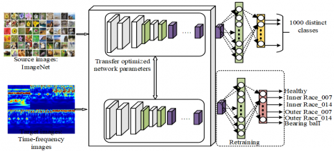
The Alexnet structure given in Figure 8 is trained on a large data set known as ImageNet. This dataset has 1000 classes of millions of samples. As noted in many studies, it is difficult to obtain such data size. Transfer learning is used to overcome this problem, in which the hidden layer that extracts features between the lower layers is similar to the Gabor filter, whereas the upper layers carry information with specific properties to the original classification task. By taking optimized network parameters for 1000 classes, transfer learning is applied to diagnostics, which is a more specific classification problem. Instead of creating a new convolutional neural network with random weights, the network can be adapted for specific classification problems using an optimized and pre-trained convolutional neural network. The structure of transfer learning is given in Figure 9.
As shown in Figure 9, the transfer learning algorithm retrieves optimized network parameters in the lower layers of the actual network. Although the actual network is bent to classify 1000 objects, only the last layers in the transfer learning are retrained.
The performance of the classifier is obtained using some measures obtained from the confusion matrix. A confusion matrix for a classifier with four classes is given in Table 1.
In Table 1, TPxx represents the number of correctly classified samples for class x, and NIx is the total number of samples classified as label x. FPxy represents the number of incorrectly classified samples for class label y classified as label x. The parameters NIx and NTx represent the total number of samples classified as x and test samples with true label x, respectively. To accurately evaluate the performance of our method, the confusion matrix is given for each classifier. Four measures such as precision (P), recall (R), accuracy rate (AR), and F1 score (F1) are calculated on each class. These measures are calculated as follows:
$P=\frac{1}{C} \sum_{i=1}^{C} \frac{T P_{i i}}{N_{i}}$ (18)
$R=\frac{1}{C} \sum_{i=1}^{C} \frac{T P_{i i}}{N T_{i}}$ (19)
$F_{1}=2 * \frac{P * R}{P+R}$ (20)
$A R=\frac{\sum_{i=1}^{C} T P_{i i}}{t o t a l}$ (21)
The proposed fault diagnosis approach was confirmed based on the dataset obtained from bearing data center at Case Western Reserve University (CWRU) [44]. The experimental setup consists of a 2-hp motor, a torque transducer, and a dynamometer. The test shaft bearings are connected to the motor shaft. Common faults in the induction motor such as inner race, outer race, and ball bearing are manufactured in different severities. The experimental setup of this bearing is given in Figure 10.
Figure 10. Experimental setup [44]
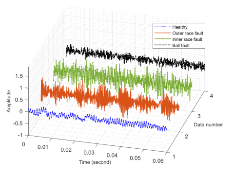
SKF type bearing is used on the fan and drive side of the motor, operated at a four different speed and four different loads with a dynamometer. The motor speed for each operating condition is collected using a torque transducer/encoder. The sampling rate of vibration data is 12 kHz, and the signals are acquired using a 16 channel data acquisition card. The vibration sensors are installed perpendicular to the top of the housing for both the fan and the drive end of the motor. The raw vibration signals are given in Figure 11 for healthy state, inner race fault, ball fault, and outer race fault cases, which are developed from CWRU bearing dataset.
Figure 11. Raw vibration signals for healthy and three fault conditions
As shown in Figure 11, the vibration signals of the health condition and the ball fault are in closed proximity to each other. One healthy and five fault conditions are considered. The healthy condition is labeled as C1. Two inner race faults have different fault severities. For the inner race fault, two fault severities are generated, one with an inner race of 0.07 inch (labeled as C2) and the second with a 0.14 inch (labeled as C3) wear. Two fault conditions of the same magnitude similar to the inner race fault are generated for the outer ring, which is labeled C4 and C5, respectively. The last fault condition is related to the ball fault labeled as C6. The descriptions of collected bearing data are given in Table 2.
Table 2. The used dataset for bearing faults
|
Fault type |
Fault size (inch) |
Rotation Speed (rpm) |
Fault class |
|||
|
1730 |
1750 |
1772 |
1797 |
|||
|
Healthy |
None |
R |
R |
R |
R |
C1 |
|
Inner race |
0.007 |
R |
R |
R |
R |
C2 |
|
0.014 |
R |
R |
R |
R |
C3 |
|
|
Outer race |
0.007 |
R |
R |
R |
R |
C4 |
|
0.014 |
R |
R |
R |
R |
C5 |
|
|
Ball |
0.007 |
R |
R |
R |
R |
C6 |
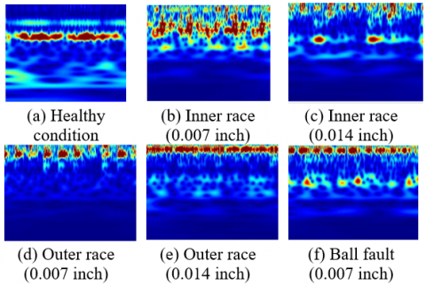
In Table 2, all fault conditions are taken into consideration, and fault detection is at four different speeds. The vibration signals were converted to the TF domain using continuous wavelet analysis. The TF representations of the healthy and faulty conditions of bearing signals are given in Figure 12.
Figure 12. TF representation of vibration signals for different working conditions
In Figure 12, the continuous wavelet transform was applied to vibration signals. The signal size is selected as 1024 samples without overlapping. After TF representations of each condition have been obtained, they are converted to grayscale images. For texture classification, coHOG descripts the occurrence of HOG in a given texture image. The parameters of coHOG such as a number of orientation bins and offsets are selected as 8 with a 4x4 squared grid and 6, respectively. The size of the feature vector is obtained as 128. The dimension of the feature vector became 3072 for coHOG method. The obtained features for a healthy and fault condition are revealed in Figure 13.
Figure 13. Feature vector for vibration signal
As shown in Figure 13, the feature vectors of healthy and faulty conditions are quite different from each other. Each feature vector was normalized using z-score normalization. The performance of the sparse classifier is extensively evaluated using CWRU bearing dataset.
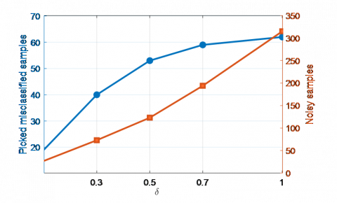
After the feature extraction, the obtained features are given to the ELMSRC classifier, and the motor condition is classified. The data set consists of a total of 3908 samples, and the performance of the classifier depends on the appropriate setting of the $\delta$ parameter. This parameter is set to capture incorrectly classified data and to classify the data according to the SRC procedure. This parameter may increase the number of noisy samples, although it may capture incorrectly classified samples when incorrectly selected. The number of neurons in the hidden layer of the ELM classifier is selected as 1000, and the sigmoidal function is used as the activation function. The ELM method has misclassified 70 of 1173 test samples. Figure 14 shows the number of picked misclassification samples and noisy samples of the ELMSRC for different $\delta$ parameters.
Figure 14. Picked and noisy samples from ELMSRC output with different $\delta$
As shown in Figure 14, the number of picked misclassified samples increases, whereas the number of noisy samples increases for different $\delta$ parameters. When the parameter $\delta$ is selected as 0.5, the gap between the number of noisy samples and the number of picked misclassified samples is the largest. Therefore, the parameter $\delta$ was chosen as 0.5. In this study, each signal consists of 1000 samples. The size of the training set obtained was 3908 for six classes. Samples were taken under each working speed and load for a healthy condition. Ten-fold cross-validation was used to avoid over-learning and to improve generalization during training. The overall confusion matrix is given in Table 3 for all test run.
Table 3. Confusion matrix of ELMSRC for 10 different test subsets
|
|
True classes |
||||||
|
Predicted class |
|
C1 |
C2 |
C3 |
C4 |
C5 |
C6 |
|
C1 |
466 |
|
1 |
|
|
6 |
|
|
C2 |
|
476 |
|
|
|
|
|
|
C3 |
5 |
|
453 |
|
|
14 |
|
|
C4 |
|
|
|
1657 |
|
|
|
|
C5 |
|
|
|
|
356 |
|
|
|
C6 |
27 |
|
2 |
|
|
445 |
|
According to the complexity matrix in Table 3, the classifier seems to confuse C1 and C6. The performance of the proposed method was obtained according to classification accuracy, sensitivity, recall, and F1 measurement. Table 4 shows the performance of HOG and coHOG when using ELMSRC according to both HOG and coHOG methods.
Table 4. Performance evaluation results for two feature extraction method
|
PERFORMANCE MEASURES |
FEATURE EXTRACTION METHOD |
|
|
HOG(%) |
coHOG(%) |
|
|
Precision |
92.67 |
98.20 |
|
Recall |
93.20 |
98.08 |
|
F1 |
92.93 |
98.13 |
|
Accuracy |
94.67 |
98.59 |
As shown in Table 1, when coHOG features were used in the classification stage, a better accuracy rate and lower false alarms were obtained compared to HOG.
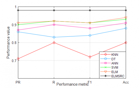
The results were compared with other well-known machine learning techniques to show the effectiveness of the proposed ELMSRC classifier. For this purpose, artificial neural networks (ANN), support vector machines (SVM), decision trees (DT), ELM, and k-nearest neighbor algorithm (KNN) were trained with obtained coHOG features. The parameters were adjusted to obtain the best performance from each method. A three-layer feedforward neural network was selected, and the number of neurons in the hidden layer was selected as 20. Sigmoid activation function was used in this layer. The Gaussian kernel was selected for SVM, and the kernel scale was selected as 36. In DT, the Gini index was used as a split criterion, and the maximum split number was determined as 100. In the ELM, 1000 neurons were used in the middle layer. Finally, the KNN parameter is taken as 10, using the Euclidean distance metric. The comparison results are given in Figure 15.
Figure 15. The performance evaluation of classifiers
As shown in Figure 15, the proposed classifier yielded the best performance on the data set. The performance metrics of ELM and SVM are similar. The precision and accuracy of ELM were higher than those of SVM. Both KNN accuracy and other performance metric are the lowest compared with other classifiers.
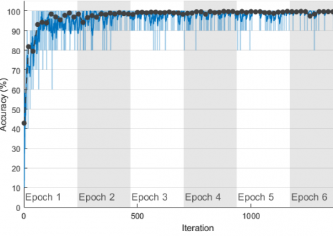
TF images representing different motor conditions were trained with the Alexnet deep learning model in order to show the effectiveness of the proposed feature extraction method. For this process, a transfer learning algorithm was utilized on a pre-trained Alexnet network. Some parameters of Alexnet architecture must be adjusted for transfer learning. The parameters of transfer learning are given in Table 5.
Table 5. Parameters of transfer learning
|
Parameter |
Value |
|
Network input size |
227x227x3 |
|
Batch size |
10 |
|
Max epochs |
6 |
|
Iterations per epoch |
234 |
|
Initial learning rate |
1e-4 |
|
Validation frequency |
3 |
The deep convolutional network was trained on a desktop computer with a 6GB GPU Card using the parameters given in Table 5. Figure 16 shows graphs of training accuracy and loss.
(a) Training accuracy rate
(b) Training loss
Figure 16. The performance of Alexnet on same dataset
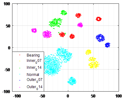
(a) Activation of Pool5
(b) Activation of fc7
Figure 17. t-SNE visualization of feature maps extracted from pool5 and fc7 layers
From the training results in Figure 16, after a certain iteration, the training and validation performance is close to 100%, and the loss value is close to zero. The total performance of the deep learning algorithm was 99.45%. This indicates that the used data preprocessing and TF representation are the correct choices. The t-SNE visualization of the feature map extracted with Alexnet is given to determine how the transfer learning of the same images looks in different layers. Figure 17 shows the visualization results for pool5 and fc7 layers.
As shown in Figure 17, healthy and faulty conditions are clearly distinguished. On the other hand, the shaft bearing ball failure and some parts of Outer_14 and Inner_14 time-frequency with each other. The results show that the images obtained to demonstrate healthy and faulty conditions successful express different faulty conditions. The proposed method is compared with other deep learning and traditional intelligent computing techniques proposed by previous studies that use the same benchmark data set. For this purpose, the proposed method was compared with well-known traditional intelligent computational techniques such as SVM and ANN. The performance of the proposed method was also compared with two different CNNs. The comparison was made according to the accuracy rates, and the results are given in Table 6.
Table 6. Comparison of the proposed method to different intelligent and deep learning methods
|
Reference |
Classifier |
Feature extraction |
Number of classes |
Accuracy rate |
|
[11] |
CNN |
Convert raw signals to an image |
4 |
96.75% |
|
[16] |
SVM |
Statistical feature extraction from time domain signal |
4 |
96.10% |
|
[25] |
1D CNN |
Raw signals |
6 |
93.30% |
|
[45] |
SVM ensemble |
Wavelet analysis |
4 |
89.80% |
|
[46] |
ANN |
Discrete wavelet transform with daubechies10 |
2 |
93.30% |
|
[47] |
ANN |
Convert raw signals to an image and Local binary pattern |
4 |
95.90% |
|
Proposed |
ELMSRC classifier |
Time frequency image representation and coHOG based feature extraction |
6 |
98.59% |
In conventional artificial intelligence-based diagnostic methods, the features are extracted from the raw signal using a pre-processing method. Then, classification is performed by evaluating the obtained features. Wavelet analysis, Fourier transform, and other statistical methods are used for feature extraction. The principal component analysis is applied to the obtained high dimensional data for reducing dimension. The features obtained depend on the load or operating speed, which do not provide a generalization for all fault conditions. In addition, the obtained features require knowledge of the number of balls, the inner, and outer race diameter of the motor shaft bearing. Feature selection and size reduction bring an extra cost. Although faulty conditions of convolutional neural networks are better, its disadvantage is that both computational loads are high and require large data. The conversion from the raw signal to a two-dimensional matrix, using a convolutional neural network and recording the matrix as an image, functions normally in all cases. The one-dimensional convolutional neural network is used for constant load conditions. Time-frequency representation is obtained by wavelet analysis and accurately reflected the fault information. Distinctive images for different faults and healthy conditions are obtained by using this feature extraction technique. The obtained images are considered as the basic known texture classification problem, and feature extraction is performed by coHOG method, combined with the SRC method to increase the ELM testing capability. The proposed method provides the following contributions.
In this paper, we propose an extreme learning machine and a sparse representation-based method for the diagnosis of bearing faults. The proposed method obtains the time-frequency representation image by applying continuous wavelet analysis to the raw vibration signals. The features are extracted from the TF image using the coHOG transform. The obtained features are classified by extreme learning machine and sparse representation-based method. The proposed approach is used to determine three different fault types and different fault sizes on a benchmark data set. The obtained TF images accurately represent different fault conditions. coHOG based feature extraction method use gradient orientation pairs. These blocks create histograms and represent local and global features of an image in detail. The proposed classification approach achieved 98.59% accuracy for a data set with 6 classes. The classification results demonstrate that the proposed coHOG-based feature extraction can extract distinctive features from the TF image. In addition, the proposed method does not require manual parameter setting, calculation of different frequency components, and extra sensor information. By testing bearing failures with different severity of the failure, the obtained results were close to the results of the Alexnet. Our method is also experimentally better than other methods in the literature.
[1] Faiz, J., Joksimovic, G., Ghorbanian, V. (2017). Fault diagnosis of induction motors. Institution of Engineering & Technology. https://doi.org/10.1049/PBPO108E
[2] Gao, Z., Cecati, C., Ding, S.X. (2015). A survey of fault diagnosis and fault-tolerant techniques-Part I: Fault diagnosis with model-based and signal-based approaches. IEEE Transactions on Industrial Electronics, 62(6): 3757-3767. https://doi.org/10.1109/TIE.2015.2417501
[3] Zhang, P., Du, Y., Habetler, T.G., Lu, B. (2010). A survey of condition monitoring and protection methods for medium-voltage induction motors. IEEE Transactions on Industry Applications, 47(1): 34-46. https://doi.org/10.1109/TIA.2010.2090839
[4] Liu, Y., Bazzi, A.M. (2017). A review and comparison of fault detection and diagnosis methods for squirrel-cage induction motors: State of the art. ISA Transactions, 70: 400-409. https://doi.org/10.1016/j.isatra.2017.06.001
[5] Ghorbanian, V., Faiz, J. (2015). A survey on time and frequency characteristics of induction motors with broken rotor bars in line-start and inverter-fed modes. Mechanical Systems and Signal Processing, 54-55: 427-456. https://doi.org/10.1016/j.ymssp.2014.08.022
[6] Gao, Z., Cecati, C., Ding, S.X. (2015). A survey of fault diagnosis and fault-tolerant techniques-Part II: Fault diagnosis with model-based and signal-based approaches. IEEE Transactions on Industrial Electronics, 62(6): 3768-3774. https://doi.org/10.1109/TIE.2015.2419013
[7] Wang, J., Zhang, L., Duan, L., Gao, R.X. (2017). A new paradigm of cloud-based predictive maintenance for intelligent manufacturing. Journal of Intelligent Manufacturing, 28(5): 1125-1137. https://doi.org/10.1007/s10845-015-1066-0
[8] Gandomi, A., Haider, M. (2015). Beyond the hype: Big data concepts, methods, and analytics. International Journal of Information Management, 35(2): 137-144. https://doi.org/10.1016/j.ijinfomgt.2014.10.007
[9] Paliwal, D., Choudhur, A., Govandhan, T. (2014) Identification of faults through wavelet transform vis-à-vis fast Fourier transform of noisy vibration signals emanated from defective rolling element bearings, Frontiers of Mechanical Engineering, 9: 130-141. https://doi.org/10.1007/s11465-014-0298-6
[10] Goyal, D., Choudhary, A., Pabla, B.S., Dhami, S.S. (2020). Support vector machines based non-contact fault diagnosis system for bearings. Journal of Intelligent Manufacturing, 31: 1275-1289. https://doi.org/10.1007/s10845-019-01511-x
[11] Hoang, D.T., Kang, H.J. (2019). Rolling element bearing fault diagnosis using convolutional neural network and vibration image. Cognitive Systems Research, 53: 42-50. https://doi.org/10.1016/j.cogsys.2018.03.002
[12] Helmi, H., Forouzantabar, A. (2018). Rolling bearing fault detection of electric motor using time domain and frequency domain features extraction and ANFIS. IET Electric Power Applications, 13(5): 662-669. https://doi.org/10.1049/iet-epa.2018.5274
[13] Zarei, J., Tajeddini, M.A., Karimi, H.R. (2014). Vibration analysis for bearing fault detection and classification using an intelligent filter. Mechatronics, 24(2): 151-157. https://doi.org/10.1016/j.mechatronics.2014.01.003
[14] Nayana, B.R., Geethanjali, P. (2017). Analysis of statistical time-domain features effectiveness in identification of bearing faults from vibration signal. IEEE Sensors Journal, 17(17): 5618-5625. https://doi.org/10.1109/JSEN.2017.2727638
[15] Li, Y., Dai, W., Zhang, W. (2020). Bearing fault feature selection method based on weighted multidimensional feature fusion. IEEE Access, 8: 19008-19025. https://doi.org/10.1109/ACCESS.2020.2967537
[16] Elbouchikhi, E., Choqueuse, V., Auger, F., Benbouzid, M.E.H. (2017). Motor current signal analysis based on a matched subspace detector. IEEE Transactions on Instrumentation and Measurement, 66(12): 3260-3270. https://doi.org/10.1109/TIM.2017.2749858
[17] Wang, T., Liang, M., Li, J., Cheng, W. (2014). Rolling element bearing fault diagnosis via fault characteristic order (FCO) analysis. Mechanical Systems and Signal Processing, 45(1): 139-153. https://doi.org/10.1016/j.ymssp.2013.11.011
[18] Maruthi, G.S., Hegde, V. (2015). Application of MEMS accelerometer for detection and diagnosis of multiple faults in the roller element bearings of three phase induction motor. IEEE Sensors Journal, 16(1): 145-152. https://doi.org/10.1109/JSEN.2015.2476561
[19] Attoui, I., Fergani, N., Boutasseta, N., Oudjani, B., Deliou, A. (2017). A new time–frequency method for identification and classification of ball bearing faults. Journal of Sound and Vibration, 397: 241-265. https://doi.org/10.1016/j.jsv.2017.02.041
[20] Zhang, X., Liu, Z., Wang, J., Wang, J. (2019). Time–frequency analysis for bearing fault diagnosis using multiple Q-factor Gabor wavelets. ISA Transactions, 87: 225-234. https://doi.org/10.1016/j.isatra.2018.11.033
[21] Soualhi, A., Medjaher, K., Zerhouni, N. (2015). Bearing health monitoring based on Hilbert-Huang transform, support vector machine, and regression. IEEE Transactions on Instrumentation and Measurement, 64(1): 52-62. https://doi.org/10.1109/TIM.2014.2330494
[22] Corne, B., Vervisch, B., Derammelaere, S., Knockaert, J., Desmet, J. (2018). The reflection of evolving bearing faults in the stator current’s extended park vector approach for induction machines. Mechanical Systems and Signal Processing, 107: 168-182. https://doi.org/10.1016/j.ymssp.2017.12.010
[23] Aydın, İ., Karaköse, M., Akın, E. (2015). Combined intelligent methods based on wireless sensor networks for condition monitoring and fault diagnosis. Journal of Intelligent Manufacturing, 26(4): 717-729. https://doi.org/10.1007/s10845-013-0829-8
[24] Randall, R.B., Antoni, J. (2011). Rolling element bearing diagnostics-A tutorial. Mechanical Systems and Signal Processing, 25(2): 485-520. https://doi.org/10.1016/j.ymssp.2010.07.017
[25] Eren, L., Ince, T., Kiranyaz, S. (2019). A generic intelligent bearing fault diagnosis system using compact adaptive 1D CNN classifier. Journal of Signal Processing Systems, 91(2): 179-189. https://doi.org/10.1007/s11265-018-1378-3
[26] Wen, L., Li, X., Gao, L., Zhang, Y. (2017). A new convolutional neural network-based data-driven fault diagnosis method. IEEE Transactions on Industrial Electronics, 65(7): 5990-5998. https://doi.org/10.1109/TIE.2017.2774777
[27] Randall, R.B. (2011). Vibration Based Condition Monitoring: Industrial, Aerospace and Automotive Applications. Chichester, UK: John Wiley and Sons.
[28] Luo, M., Zhang, K. (2014). A hybrid approach combining extreme learning machine and sparse representation for image classification. Engineering Applications of Artificial Intelligence, 27: 228-235. https://doi.org/10.1016/j.engappai.2013.05.012
[29] Mitra, Sanjit K. (2001). Digital Signal Processing: A Computer-Based Approach. 2nd Ed. New York: McGraw-Hill.
[30] Choraś R.S. (2014) Time-Frequency Analysis of Image Based on Stockwell Transform. In: S. Choras R. (eds) Image Processing and Communications Challenges 5. Advances in Intelligent Systems and Computing, vol. 233. Springer, Heidelberg. https://doi.org/10.1007/978-3-319-01622-1_11
[31] Moukadem, A., Ould Abdeslam, D., Dieterlen, A. (2014). Time–Frequency Analysis: The S‐transform: Time–Frequency Domain for Segmentation and Classification of Non‐Stationary Signals: The Stockwell Transform Applied on Bio‐Signals and Electric Signals, 21-59. John Wiley & Sons.
[32] Cohen, L. (1995). Time-Frequency Analysis: Theory and Applications. Englewood Cliffs, NJ: Prentice-Hall.
[33] Lilly, J.M., Olhede, S.C. (2012). Generalized Morse wavelets as a superfamily of analytic wavelets. IEEE Transactions on Signal Processing, 60(11): 6036-6041. https://doi.org/10.1109/TSP.2012.2210890
[34] Talhaoui, H., Menacer, A., Kessal, A., Tarek, A. (2018). Experimental diagnosis of broken rotor bars fault in induction machine based on Hilbert and discrete wavelet transforms. The International Journal of Advanced Manufacturing Technology, 95: 1399-1408. https://doi.org/10.1007/s00170-017-1309-7
[35] da Costa, C., Kashiwagi, M., Mathias, M.H. (2015). Rotor failure detection of induction motors by wavelet transform and Fourier transform in non-stationary condition. Case Studies in Mechanical Systems and Signal Processing, 1: 15-26. https://doi.org/10.1016/j.csmssp.2015.05.001
[36] Jawadekar, A., Paraskar, S., Jadhav, S., Dhole, G. (2014). Artificial neural network-based induction motor fault classifier using continuous wavelet transform. Systems Science & Control Engineering: An Open Access Journal, 2(1): 684-690. https://doi.org/10.1080/21642583.2014.956266
[37] Zarei, J., Poshtan, J. (2007). Bearing fault detection using wavelet packet transform of induction motor stator current. Tribology International, 40(5): 763-769. https://doi.org/10.1016/j.triboint.2006.07.002
[38] Cohen L. (2003). The wavelet transform and time-frequency analysis. In: Debnath L. (eds) Wavelets and Signal Processing, Boston, pp. 3-22.
[39] Pukhova, V., Gorelova, E., Ferrini, G., Burnasheva, S. (2017). Time-frequency representation of signals by wavelet transform. IEEE Conference of Russian Young Researchers in Electrical and Electronic Engineering, St. Petersburg, pp. 715-718. https://doi.org/10.1109/EIConRus.2017.7910658
[40] Dalal, N., Triggs, B. (2015). Histograms of oriented gradients for human detection. IEEE Computer Society Conference on Computer Vision and Pattern Recognition, San Diego, pp. 886-893. https://doi.org/10.1109/CVPR.2005.177
[41] Watanabe, T., Ito, S., Yokoi, K. (2009). Co-occurrence Histograms of Oriented Gradients for Pedestrian Detection. In: Wada T., Huang F., Lin S. (eds) Advances in Image and Video Technology. PSIVT 2009. Lecture Notes in Computer Science, vol. 5414. Springer, Berlin, Heidelberg. https://doi.org/10.1007/978-3-540-92957-4_4
[42] Huang, G.B., Zhou, H., Ding, X., Zhang, R. (2011). Extreme learning machine for regression and multiclass classification. IEEE Transactions on Systems, Man, and Cybernetics, Part B, 42(2): 513-529. https://doi.org/10.1109/TSMCB.2011.2168604
[43] Krizhevsky, A., Sutskever, I., Hinton, G.E. (2017). Imagenet classification with deep convolutional neural networks. Communications of the ACM, 60(6): 84-90. https://doi.org/10.1145/3065386
[44] Case western University Bearing Data Center. https://csegroups.case.edu/bearingdatacenter/home, accessed on Sept. 10, 2020.
[45] Hu, Q., He, Z., Zhang, Z., Zi, Y. (2007). Fault diagnosis of rotating machinery based on improved wavelet package transform and SVMs ensemble. Mechanical Systems and Signal Processing, 21(2): 688-705. https://doi.org/10.1016/j.ymssp.2006.01.007
[46] Konar, P., Chattopadhyay, P. (2011). Bearing fault detection of induction motor using wavelet and Support Vector Machines (SVMs). Applied Soft Computing, 11(6): 4203-4211. https://doi.org/10.1016/j.asoc.2011.03.014
[47] Kaplan, K., Kaya, Y., Kuncan, M., Mi̇naz, M.R., Ertunç, H.M. (2019). An improved feature extraction method using texture analysis with LBP for bearing fault diagnosis. Applied Soft Computing, 87: 1-13. https://doi.org/10.1016/j.asoc.2019.106019