Xiaoping Cao | Tao Li | Jiawei Bai* | Zhikai Wei
© 2020 IIETA. This article is published by IIETA and is licensed under the CC BY 4.0 license (http://creativecommons.org/licenses/by/4.0/).
OPEN ACCESS
The crack identification and classification are essential to the discovery and maintenance of early defects in concrete members. This paper designs a novel method that supports accurate identification and classification of surface cracks on concrete members. Specifically, each sample image was preprocessed through cropping and neighborhood operation, subject to gray adaptive thresholding, and further processed based on morphological gradient and local gray value dissimilarity. Next, the Gauss-Laplace algorithm was employed to extract the contours of the surface cracks, and each image was matched with the normalized crack templates one by one. Finally, a densely connected neural network of transfer learning was introduced to rapidly classify the surface cracks on concrete members. The effectiveness and accuracy of our method were fully demonstrated through experiments. The research findings provide a reference for surface crack identification and classification in other fields.
surface cracks on concrete members, image processing, image segmentation, crack identification and classification
During infrastructure construction, concrete members could be damaged and cracked for reasons of careless operation, excess load, etc. The cracking threatens the structure and bearing capacity of the building structure [1-5]. The surface cracks on concrete member may arise from various factors. Currently, these cracks are mostly detected and maintained manually. These manual interventions tend to be complex, dangerous, and inaccurate [6-9]. For functional reliability of concrete members, it is critical to identify and classify the surface cracks in an accurate and efficient manner [10-12].
At present, some image processing-based methods have been applied to detect the cracks on concrete buildings like bridges and highways. In these methods, surface crack images are collected by multi-function inspection vehicles, and subjected to preprocessing, segmentation and crack identification; Finally, the type of cracks and the degree of building damages are judged and predicted manually [13-18]. Based on deep learning, Chen et al. [19] proposed a robust, automatic crack detection method, capable of mitigating the effect of building shadows on images and effectively suppressing noise. In view of crack skeleton, Chen et al. [20] also developed an efficient edge detection technique, which achieves high accuracy by removing the areas with similar gray values. Drawing on approximate watershed algorithm, Emmanuel Maggiori et al. [21] constructed a novel crack detection and penetration model: the cracks are identified rapidly and accurately by simulating the fractal law of liquid penetration under stress. Nicolas et al. [22] put forward an automatic road crack detection method, which effectively detects road surface cracks, using structured random forest algorithm and multi-feature crack classifier.
To identify and classify the surface cracks on concrete members, the digital image processing technique must have high accuracy in processing and classification and a wide application range [23-25]. This paper puts forward a novel method that supports accurate identification and classification of surface cracks on concrete members. Firstly, each sample image was cropped, and subject to neighborhood operation, achieving the effect of Gaussian filtering. The preprocessed image was subject to gray adaptive thresholding based on grayscale probability, and removed of interfering pixels (e.g. noise and burrs) based on morphological gradient and local gray value dissimilarity. After that, the Gauss-Laplace algorithm was adopted to extract the contours of the surface cracks, and each image was matched with the normalized crack templates one by one. Finally, a densely connected neural network of transfer learning was introduced to rapidly classify the surface cracks on concrete members. Our method was proved effective through experiments.
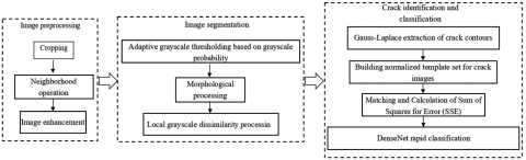
As shown in Figure 1, the proposed method can be broken down into three stages: image preprocessing, image segmentation, and crack identification and classification.
To realize fast recognition and classification, the collected surface images on concrete members were preprocessed through cropping and neighborhood operation, based on the image enhancement technique for surface cracks on concrete members. The preprocessing simplifies the image information to the greatest possible extent. Through image preprocessing, the redundant information could be removed, and the useful information could be enhanced, laying the basis for reliable crack classification. During the preprocessing, image enhancement was conducted to highlight the surface crack features, making the cracks more noticeable.
Figure 1. Workflow of our method
Here, every original image of surface crack on concrete members was binarized by Otsu’s method. The image was cropped along the bounding box in the white area into image I(x, y) of the size A×B, where x=0, 1, 2…A-1 and y=0, 1, 2…B-1. The cropped image was fitted as a straight line along the pixels of the bounding box. Based on the preset length a and width b, the fitted line was translated to construct a rectangular template M of the size a×b.
Each pixel in the cropped image was subject to neighborhood operation:
${I}'(x,y)=\sum\limits_{a,b}{I(x+a,y+b)\cdot M(a,b)}\text{ }$ (1)
where, I(x, y) is the value of a pixel in the original image; I¢(x, y) is the value of that pixel after neighborhood operation (neighborhood pixel value); M(a, b) is the neighborhood operation function. The neighborhood pixel values were taken as the initial values for the next iteration of neighborhood operation. Then, the neighborhood pixel values were subject to weighted summation by:
${I}'\left( x,y \right)=\frac{\sum\limits_{c,d}{(\sum\limits_{a,b}{I(x+a,y+b)M(a,b)})\delta (c,d)}}{\sum\limits_{c,d}{\delta (c,d)}}$ (2)
where, δ(c, d) is the weight coefficient dependent on the kernel values of the domain of definition of range. If the gray value difference is small among the pixels in the neighborhood, the weighted summation is comparable to Gaussian filtering; if the gray value difference is large, the weighted summation has a limited effect on the image state.
To effectively extract the crack defects, it is necessary to segment every preprocessed image of surface crack on concrete members. The most popular methods for image segmentation include the Otsu’s method and Niblack’s method. After neighborhood operation, the gray values of pixels are concentrated on the image. In this case, the Otsu’s method may overlook the specific information of cracks, while the Niblack’s method needs to be coupled with a suitable denoising method.
The absolute difference between a pixel of the original image and the corresponding pixel of the image processed by neighborhood operation was taken as the high-frequency component h(x, y) of that pixel:
$h\left( x,y \right)=\left| {I}'\left( x,y \right)-I\left( x,y \right) \right|$ (3)
Let G be the grayscale of I(x, y). Then, the probability pl that the grayscale of h(x, y) is l can be estimated by:
${{p}_{l}}=\frac{h\left( x,y \right)}{a\times b}$ (4)
$\sum\limits_{l=0}^{G-1}{{{p}_{l}}=1}$ (5)
where, a×b is the size of the neighborhood. Based on grayscale, the high-frequency components of pixels in the surface crack image were divided into two classes: background region of interest (ROI) (grayscale: 0~g-1) and target ROI (grayscale: g~G-1), where g is gray value. The pixel sets of the two classes are {I(x, y)<g} and {I(x, y)≥g}, respectively. The grayscale probabilities of the two classes can be respectively calculated by:
${{\mu }_{1}}=\sum\limits_{l=0}^{g-1}{{{p}_{l}}}\text{ }$ (6)
${{\mu }_{2}}=\sum\limits_{l=g}^{G-1}{{{p}_{l}}}\text{ }$ (7)
Since μ1+μ2=1, the mean gray value of h(x, y) is the sum of the gray scales of the two ROIs:
$T={{t}_{1}}(g)+{{t}_{2}}(g)=\sum\limits_{l=1}^{g-1}{l}\cdot \frac{{{p}_{l}}}{{{\mu }_{1}}}+\sum\limits_{l=g}^{G-1}{l}\cdot \frac{{{p}_{l}}}{{{\mu }_{2}}}$ (8)
Let T be the gray adaptive threshold with grayscale probability that segments the image h(x, y). Then,
${I}'(x,y)=\left\{ \begin{align} & 1,h(x,y)\ge T \\ & 0,h(x,y)<T \\ \end{align} \right.(x,y)\in M$ (9)
After thresholding, the image contains lots of discrete noises and burrs on crack edges, which greatly disturb the crack identification. Here, these interfering pixels are removed based on morphological gradient and local gray value dissimilarity.
Let B(x, y) be the rectangular structural element that determines the performance of the gray morphological gradient operator. Then, the expansion and corrosion can be respectively expressed as:
$\left\{ \begin{matrix} \left( I\oplus B \right)\left( x,y \right)=\max \left\{ I\left( x-i,y-j \right)+b\left( i,j \right) \right\} \\ \left( I\Theta B \right)\left( x,y \right)=\min \left\{ I\left( x-i,y-j \right)-b\left( i,j \right) \right\} \\ \end{matrix} \right.$ (10)
The expansion-first closing operation and corrosion-first expansion operation can be respectively defined as:
$\left\{ \begin{matrix} I\bullet B=\left( I\oplus B \right)\Theta B \\ I\circ B=\left( I\Theta B \right)\oplus B \\ \end{matrix} \right.$ (11)
On crack boundaries, the gray morphological gradient operator can be described as:
$M=\left( I\oplus B \right)\left( x,y \right)-\left( I\Theta B \right)\left( x,y \right)$ (12)
The noises of the image were processed by the gray morphological gradient operator. If the gray value assigned to B(x, y) is too large, the peak gradient will not match with the image boundary. If the gray value is relatively small, the crack edges could be processed well, but the processing effect is greatly affected by noises. To prevent the coordinates of edge pixels from moving out of boundary, (2a¢+1)×(2b¢+1) was taken as the calculation window, and I(x, y) was expanded outward by a¢×b¢ pixels. The dissimilarity feature can be computed by:
$D$ iss $(x, y)=\left|\sum_{n=1}^{n_{1}}\right| I(x, y)-t_{1}(g)\left|/ n_{1}-\sum_{n=1}^{n_{2}}\right| I(x, y)-t_{2}(g)\left|/ n_{2}\right|$ (13)
where, n1 and n2 are the number of pixels in background ROI and target ROI of the calculation window, respectively. The corresponding gay value can be predicted as:
${{O}_{est}}=\frac{1}{A\times B}\sum\limits_{i,j\in M}{D\text{iss}\left( x,y \right)}$ (14)
where, M is the set of all pixels with nonzero gray values in h(x, y). Taking the predicted gray value as the threshold, the crack pixels in the image were processed to eliminate the interfering pixels. If a pixel has a greater dissimilarity than the threshold, the gray value will not be changed; otherwise, the gray value will be reset to one.
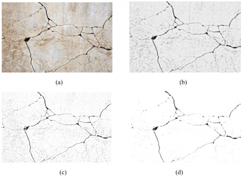
Figure 2 compares the image processing results under different calculation windows. It can be seen that the smaller the calculation window, the more interfering pixels are eliminated. After all pixels had been processed, the boundaries became smooth, the interfering pixels were separated from crack pixels, and some interfering pixels were deleted.
Figure 2. Results of image segmentation
In essence, crack identification and classification are to extract the defect features of cracks, that is, distinguish crack pixels from non-crack pixels based on data information. In the preceding sections, each sample image was preprocessed, subject to gray adaptive thresholding, and removed of interfering pixels based on morphological gradient and local gray value dissimilarity. Then, it is necessary to effectively distinguish between crack pixels and non-crack pixels by crack features.
There are four typical types of surface cracks on concrete members, each has their unique causes: the transverse cracks perpendicular to member surface induced by pressure or thermal expansion/contraction; the shear cracks induced by member movement under vibration or pressure; oblique cracks on wall surface induced by foundation settlement or thermal expansion/contraction; cross cracks induced by sudden external stress. Due to the complex causes of cracking, the actual cracks often cover multiple types. Hence, it is not suitable to process crack images with a fixed threshold.
In this paper, Gauss-Laplace algorithm is used to extract the contours of the surface cracks on concrete members, and normalize the crack templates; the image was matched with templates one by one, revealing the salient features of the surface cracks. Considering the complex cracks and chaotic noises on concrete members, the authors introduced a densely connected neural network of transfer learning to rapidly classify the surface cracks.
4.1 Surface crack identification
The reciprocal directional Gaussian filter and the Laplace edge sharpening filter can be respectively defined as:
$G(x)=\frac{\rho^{2}[\cos \theta, \sin \theta]}{\lambda^{2}} \cdot \frac{1}{2 \pi \lambda^{2}} \exp \left(-\frac{1}{2 \lambda^{2}} I^{T} R_{\theta}\left(\begin{array}{cc}\rho^{2} & 0 \\ 0 & \rho^{-2}\end{array}\right) R_{\theta}(I)\right)$ (15)
$\nabla^{2} I(x, y)=I(x+1, y)+I(x-1, y)+I(x, y+1)+I(x, y-1)-4 I(x, y)$ (16)
where, ρ is the compression or stretching ratio coefficient in each direction; λ is the scale factor; IT is the transposition of pixel coordinates; Rθ is the rotation matrix. The surface crack contours were detected through the smoothing and denoising by Gauss-Laplace filter. The obtained contour information includes crack textures and boundaries.
To narrow the physical differences between the feature components within salient features, the four types of crack templates were normalized based on the salient feature components. Firstly, a crack template set was constructed Model=[Model1, Model2, …Model4]. Then, a sample Modeli was selected randomly. Let Modelimax, Modelimin, and Modeliav be the maximum, minimum and average of the feature component values of Modeli, respectively. Then, the component values were normalized into [-1, 1] by:
$M o \operatorname{del}_{i}^{\prime}(x, y)=\frac{4\left(\operatorname{Model}_{i}(x, y)-M \operatorname{odel}_{i a v}(x, y)\right)}{\sum_{i=1}^{4}\left(M \operatorname{odel}_{i}(x, y)-M \operatorname{odel}_{i a v}(x, y)\right)}$ (17)
Or, the component values of all crack features were normalized into [0, 1] by:
$Model_{i}^{'}(x,y)=\frac{|Mode{{l}_{i}}(x,y)-Mode{{l}_{i\min }}|||}{Modelode{{l}_{i{{\min }_{i\max }}}}}$ (18)
The processed image was matched with the crack templates Modeli one by one, revealing all the pixels belong to cracks. During template matching, the sum of squares for error (SSE) was calculated between the processed image pixels and template pixels:
$E(x, y)=\sum_{k=0}^{c-1} \sum_{l=0}^{p-1}\left[I(x+k, y+l)-M \operatorname{odel}_{i}(x, y)\right]^{2}$ (19)
The above formula can be simplified as:
$E(x,y)=\sum\nolimits_{k=0}^{C-1}{\sum\nolimits_{l=0}^{D-1}{{{[I(x+k,y+l)]}^{2}}}}-2\sum\nolimits_{k=0}^{C-1}{\sum\nolimits_{l=0}^{D-1}{[I(x+k,y+l)]}}Mode{{l}_{i}}(x,y)+\sum\nolimits_{k=0}^{C-1}{\sum\nolimits_{l=0}^{D-1}{{{[Mode{{l}_{i}}(x,y)]}^{2}}={{E}_{O}}(x,y)-2}}{{E}_{O-M}}(x,y)+{{E}_{M}}(x,y)$ (20)
where, EO(x, y) and EO-M(x, y) are the positive correlation error and cross-correlation error generated when the processed image and crack templates were matched on the size of C×D, respectively. The position of each crack pixel was estimated according to EO(x, y), and EO-M(x, y).
4.2 Surface crack classification
In our research, the surface cracks are classified based on the correlation errors generated in the matching between processed image and crack templates. Based on the densely connected neural network DenseNet, the first four trained dense blocks were constructed on ImageNet dataset, and adopted as a four-dimensional (4D) fully-connected layer in crack identification and classification. The new classifier updates the correlation errors by the cross-entropy loss function:
$E^{\prime}(x, y)=\sum_{k=0}^{C-1} \sum_{l=0}^{D-1} I(x+k, y+l) \log M \operatorname{odel}(x, y)$ (21)
The classifier uses the stochastic gradient descent function to train the classification network. The weight coefficient was set to represent the learning rate of the u-th node on the t-th layer of the classifier. During the classification training, the first dense blocks of the DenseNet were frozen, and the convolution layers and pooling layers were finetuned. These operations were repeated until the classifier started to converge. Then, the output of the last dense block was extracted, and imported to the global average pooling in the classification layer. The output of that layer was converted into the classification probability by the Softmax function, and outputted as the classification result of the surface cracks on concrete members.
Our experiments were carried out in Visual Studio 2020 with a computer (CPU: Intel® Core™ i7-9700K Processor, 3.1 GHz; memory: 16GB) running on Windows 10. The software environment is Open Source Computer Vision (OpenCV) and C++, a general-purpose programming language.
Our image segmentation method was applied to process different types of surface cracks on concrete members. Figure 3 compares the original images with the images processed based on morphological gradient and local gray value dissimilarity. The comparison shows that, even if the cracks are formed under complex reasons, the interfering pixels in local dark areas were effectively removed by our method.
Figure 3. Image segmentation effects on different types of cracks
Then, the surface cracks on concrete members were classified by cracking causes into ten categories: improper operation, freezing, inadequate concrete strength, pressure effect, thermal expansion/shrinkage, rebar corrosion, foundation settlement, seismic action, fire, and improper use of materials.
Figures 4 and 5 compare the Niblack’s method and our image segmentation method in denoising effect and the accuracy of salient feature extraction on different types of cracks. It can be seen that our method extracted salient features more accurately and reduced noise rate more effectively than the Niblack’s method.
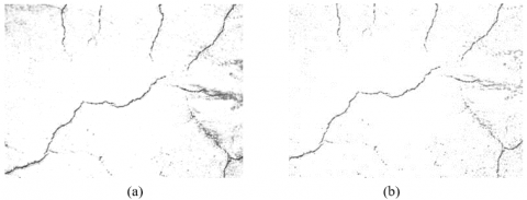
Next, our method was adopted to process an image with weak crack information and small inter-pixel grayscale difference. As shown in Figure 6, the salient features extracted by our method were continuous and complete.
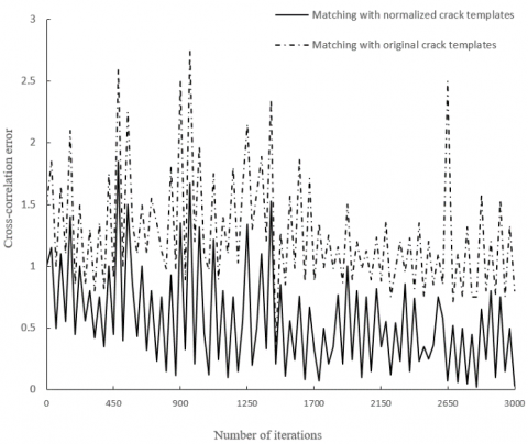
Figure 7 displays the cross-correlation error curves before and after the normalization of crack templates. Obviously, the image-template matching produced a smaller cross-correlation error after the normalization. Through 3,000 rounds of training, the matching error was reduced to the desired range.
Figure 4. Comparison of denoising effect
Figure 5. Comparison of the accuracy of salient feature extraction
Figure 6. Contour extraction effect of our method
Figure 7. Cross-correlation error curves
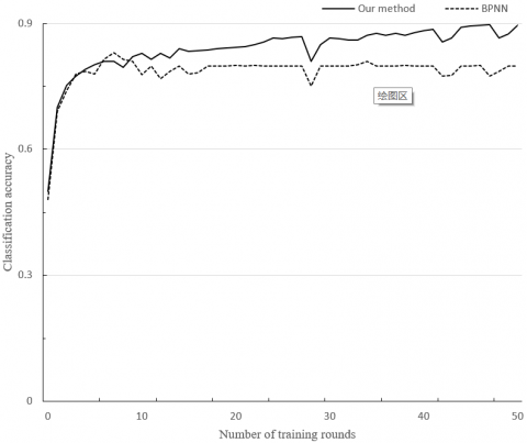
Table 1 lists the classification results of the transfer learning-based ResNet on the 10 kinds of crack images. The classification results were desirable, thanks to the saliency of crack features being extracted. Figure 8 compares the classification accuracies of our method and the backpropagation neural network (BPNN), a traditional deep convolutional neural network (D-CNN). It can be seen that our method, which relies on transfer learning, achieved higher classification accuracy than the BPNN (80%).
Table 1. Classification results on different kinds of cracks
|
Type |
Number of training rounds |
Sample size |
Accuracy /% |
|
1 |
146 |
520 |
92.35 |
|
2 |
153 |
607 |
96.42 |
|
3 |
141 |
498 |
97.52 |
|
4 |
155 |
541 |
89.75 |
|
5 |
150 |
612 |
95.43 |
|
6 |
168 |
523 |
91.51 |
|
7 |
154 |
458 |
90.47 |
|
8 |
165 |
498 |
94.22 |
|
9 |
139 |
546 |
96.57 |
|
10 |
158 |
468 |
90.24 |
Figure 8. Classification accuracy curves
This paper comes up with a strategy to identify and classify the surface cracks on concrete members. Firstly, each original image was cropped and subject to neighborhood operation. The preprocessed image was segmented by gray adaptive threshold, and also processed based on morphological gradient and local gray value dissimilarity. Experimental results confirm that the image segmentation process can effectively remove interfering pixels like noises and burrs. Afterwards, the Gauss-Laplace algorithm was introduced to extract the contours of the surface cracks, and each image was matched with the normalized crack templates one by one. Further experiments show that the image-template matching produced a smaller cross-correlation error after the normalization. In addition, the DenseNet of transfer learning was adopted to rapidly classify the surface cracks on concrete members. The experiments on 10 kinds of crack images prove that our method realized an average classification accuracy of above 90%.
[1] Kim, H., Lee, J., Ahn, E., Cho, S., Shin, M., Sim, S.H. (2017). Concrete crack identification using a UAV incorporating hybrid image processing. Sensors, 17(9): 2052. https://doi.org/10.3390/s17092052
[2] Harmouche, J., Delpha, C., Diallo, D., Le Bihan, Y. (2016). Statistical approach for nondestructive incipient crack detection and characterization using Kullback-Leibler divergence. IEEE Transactions on Reliability, 65(3): 1360-1368. https://doi.org/10.1109/TR.2016.2570549
[3] Wu, L., Mokhtari, S., Nazef, A., Nam, B., Yun, H.B. (2016). Improvement of crack-detection accuracy using a novel crack defragmentation technique in image-based road assessment. Journal of Computing in Civil Engineering, 30(1): 04014118. https://doi.org/10.1061/(ASCE)CP.1943-5487.0000451
[4] Kim, H., Ahn, E., Cho, S., Shin, M., Sim, S.H. (2017). Comparative analysis of image binarization methods for crack identification in concrete structures. Cement and Concrete Research, 99: 53-61. https://doi.org/10.1016/j.cemconres.2017.04.018
[5] Harmouche, J., Delpha, C., Diallo, D., Le Bihan, Y. (2016). Statistical approach for nondestructive incipient crack detection and characterization using Kullback-Leibler divergence. IEEE Transactions on Reliability, 65(3): 1360-1368. https://doi.org/10.1109/TR.2016.2570549
[6] Marindra, A.M.J., Tian, G.Y. (2018). Chipless RFID sensor tag for metal crack detection and characterization. IEEE Transactions on Microwave Theory and Techniques, 66(5): 2452-2462. https://doi.org/10.1109/TMTT.2017.2786696
[7] He, L.L., Zhu, H., Gao, Z.X. (2018). A novel asphalt pavement crack detection algorithm based on multi-feature test of cross-section image. Traitement du Signal, 35(3-4): 289-302. https://doi.org/10.3166/TS.35.289-302
[8] Shi, W., Caballero, J., Huszár, F., Totz, J., Aitken, A.P., Bishop, R., Rueckert, D., Wang, Z. (2016). Real-time single image and video super-resolution using an efficient sub-pixel convolutional neural network. In Proceedings of the IEEE Conference on Computer Vision and Pattern Recognition, pp. 1874-1883. https://doi.org/10.1109/CVPR.2016.207
[9] Badrinarayanan, V., Kendall, A., Cipolla, R. (2017). Segnet: A deep convolutional encoder-decoder architecture for image segmentation. IEEE Transactions on Pattern Analysis and Machine Intelligence, 39(12): 2481-2495. https://doi.org/10.1109/TPAMI.2016.2644615
[10] Chen, L.C., Papandreou, G., Schroff, F., Adam, H. (2017). Rethinking atrous convolution for semantic image segmentation. arXiv preprint arXiv:1706.05587.
[11] Chen, L.C., Zhu, Y., Papandreou, G., Schroff, F., Adam, H. (2018). Encoder-decoder with atrous separable convolution for semantic image segmentation. In Proceedings of the European Conference on Computer Vision (ECCV), pp. 801-818.
[12] Amirul Islam, M., Rochan, M., Bruce, N.D., Wang, Y. (2017). Gated feedback refinement network for dense image labeling. In Proceedings of the IEEE Conference on Computer Vision and Pattern Recognition, pp. 3751-3759.
[13] Zhou, Z., Siddiquee, M.M.R., Tajbakhsh, N., Liang, J. (2018). Unet++: A nested u-net architecture for medical image segmentation. In Deep Learning in Medical Image Analysis and Multimodal Learning for Clinical Decision Support, pp. 3-11.
[14] Litjens, G., Kooi, T., Bejnordi, B.E., Setio, A.A.A., Ciompi, F., Ghafoorian, M., van der Laak, J.A.W.M., van Ginneken, B., Sánchez, C.I. (2017). A survey on deep learning in medical image analysis. Medical Image Analysis, 42: 60-88. https://doi.org/10.1016/j.media.2017.07.005
[15] Sudre, C.H., Li, W., Vercauteren, T., Ourselin, S., Cardoso, M.J. (2017). Generalised dice overlap as a deep learning loss function for highly unbalanced segmentations. In Deep Learning in Medical Image Analysis and Multimodal Learning for Clinical Decision Support, pp. 240-248. https://doi.org/10.1016/10.1007/978-3-319-67558-9_28
[16] Chikyal, N., Swamy, K.V. (2019). Performance assessment of various thyroid image segmentation techniques with consistency verification. Jour of Adv Research in Dynamical & Control Systems, 11(Sp.2): 1299-1309.
[17] Nayak, N.R., Mishra, B.K., Rath, A.K., Swain, S. (2017). Improving the efficiency of color image segmentation using an enhanced clustering methodology. In Biometrics: Concepts, Methodologies, Tools, and Applications, pp. 1788-1802. https://doi.org/10.4018/IJAEC.2015040104
[18] Bindhu, V. (2019). Biomedical image analysis using semantic segmentation. Journal of Innovative Image Processing (JIIP), 1(2): 91-101. https://doi.org/10.36548/jiip.2019.2.004
[19] Chen, L.C., Papandreou, G., Kokkinos, I., Murphy, K., Yuille, A.L. (2017). Deeplab: Semantic image segmentation with deep convolutional nets, atrous convolution, and fully connected CRFs. IEEE Transactions on Pattern Analysis and Machine Intelligence, 40(4): 834-848. https://doi.org/10.1109/TPAMI.2017.2699184
[20] Chen, L.C., Papandreou, G., Schroff, F., Adam, H. (2017). Rethinking atrous convolution for semantic image segmentation. arXiv preprint arXiv:1706.05587.
[21] Maggiori, E., Tarabalka, Y., Charpiat, G., Alliez, P. (2017). Can semantic labeling methods generalize to any city? the inria aerial image labeling benchmark. In 2017 IEEE International Geoscience and Remote Sensing Symposium (IGARSS), pp. 3226-3229. https://doi.org/10.1109/IGARSS.2017.8127684
[22] Audebert, N., Le Saux, B., Lefèvre, S. (2017). Segment-before-detect: Vehicle detection and classification through semantic segmentation of aerial images. Remote Sensing, 9(4): 368. https://doi.org/10.3390/rs9040368
[23] Liu, Y., Minh Nguyen, D., Deligiannis, N., Ding, W., Munteanu, A. (2017). Hourglass-shapenetwork based semantic segmentation for high resolution aerial imagery. Remote Sensing, 9(6): 522. https://doi.org/10.3390/rs9060522
[24] Lv, Z.Y., Shi, W., Zhang, X., Benediktsson, J.A. (2018). Landslide inventory mapping from bitemporal high-resolution remote sensing images using change detection and multiscale segmentation. IEEE Journal of Selected Topics in Applied Earth Observations and Remote Sensing, 11(5): 1520-1532. https://doi.org/10.1109/JSTARS.2018.2803784
[25] Zanetti, M., Bruzzone, L. (2017). A theoretical framework for change detection based on a compound multiclass statistical model of the difference image. IEEE Transactions on Geoscience and Remote Sensing, 56(2): 1129-1143. https://doi.org/10.1109/TGRS.2017.2759663