Guicai Yu
© 2020 IIETA. This article is published by IIETA and is licensed under the CC BY 4.0 license (http://creativecommons.org/licenses/by/4.0/).
OPEN ACCESS
The direction of arrival (DOA) is traditionally estimated by subspace algorithms. However, the computation of subspace algorithms is complicated by eigenvalue decomposition (EVD) or singular value decomposition (SVD). To simplify subspace algorithms, this paper proposes a fast one-dimensional (1D) DOA estimation algorithm for double parallel linear array (DPLA). In our algorithm, the equivalent noise subspace is constructed by processing the first column elements of the joint cross-covariance matrix (JCCM), and the DOA is estimated, using the root-multiple signal classification (MUSIC) algorithm. The algorithm effectively simplifies and speeds up the computation by eliminating EVD or SVD. Simulation results confirm that our algorithm can improve the accuracy and reduce the time of DOA estimation. The research results have great application potential in DOA estimation tasks.
direction of arrival (DOA), double parallel linear array (DPLA), joint cross-covariance matrix (JCCM), root-multiple signal classification (MUSIC) algorithm
Direction of arrival (DOA) estimation, a key issue in array signal processing, is common in various fields, namely, radar [1-3], sonar [4, 5], communications [6, 7], seismic survey [8], and radio astronomy [9]. Array antennas have been adopted in many methods to estimate the DOA, including autoregressive-moving average (ARMA) spectral analysis, maximum likelihood method, entropy spectral analysis, and eigenvalue decomposition.
Two subspace algorithms have been developed based on eigenvalue decomposition (EVD). In 1979, Schmidt proposed the multiple signal classification (MUSIC) algorithm [10-12], marking a breakthrough in DOA estimation theories. In 1986, Roy put forward the estimation of signal parameters via rotational invariance techniques (ESPRIT) algorithm [13, 14]. Based on rotational invariance of subspaces, ESPRIT algorithm eliminates the need of global search and thus reduces the computing load. The key of subspace algorithms is to obtain signal subspace or noise subspace through EVD or singular value decomposition (SVD). Either EVD or SVD incurs a huge computing load, especially in massive multiple-input and multiple-output (MIMO) systems.
To simplify subspace algorithms, many excellent methods have been designed in recent years. For example, T.A.H. Bressner et al. [15] created the single snapshot algorithm for large arrays, which divides a large array into multiple subarrays for DOA estimation. Through low-rank matrix reconstruction and Vandermonde decomposition, Tian et al. [16] designed a gridless two-dimensional (2D) DOA estimation method that improves the running speed by avoiding EVD or SVD. But the applicable scope of this method is limited to uniform and sparse rectangular arrays. For 2D DOA estimation with L-shaped array, Nie and Li [17] proposed a computationally efficient subspace algorithm (CESA), which estimates 2D DOA efficiently with three vectors made from the elements in the first column, first row and diagonal of the covariance matrix, respectively. Since the two axes of the L-shaped array are composed of uniform linear arrays (ULAs), Yan et al. [18] established a CESA-based joint cross-covariance matrix (JCCM) algorithm for one-dimensional (1D) DOA estimation with ULA. Eliminating subspace decomposition, the JCCM algorithm sets up a JCCM based on the forward and backward cross-covariance matrices of input data, reconstructs the equivalent signal subspace, and estimates the DOA by solving polynomials
Drawing on ESPRIT algorithm [19], CESA algorithm, and JCCM algorithm, this paper proposes a 1D DOA estimation algorithm with double parallel linear array (DPLA). The DPLA [20] consists of two parallel ULAs with a known spacing. The DPLA can be viewed as an array of array elements pairs, each of which contains two sensors with identical response features. In the proposed algorithm, the noise subspace is constructed by processing the first column elements of the JCCM, and the DOA of signal is obtained by solving polynomials.
The remainder of this paper is organized as follows: Section II introduces the structure and model of the DPLA; Section III explains the DPLA algorithm and analyzes its performance; Section IV compares the DPLA algorithm with others through MATLAB simulation; Section V puts forward the conclusions.
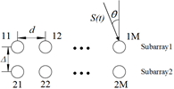
As shown in Figure 1, the DPLA contains M array element pairs, each of which has two sensors with identical response features. The DPLA can also be considered as the combination of two ULAs with the spacing of Δ. It is assumed that K≤M independent, far-field and narrowband signals $s_{1}(t), s_{2}(t), \ldots, s_{k}(t)$ are incident on the DPLA simultaneously as planar waves, and the arrival of signals is a zero-mean random process. Then, the signal sources can be differentiated by the DOA.
Figure 1. The structure of the DPLA
Suppose the arrival of signals on all array elements is a white Gaussian random process (mean: zero; variance: σ2) independent of signals. The DPLA was divided into subarray 1 and subarray 2, both of which are ULAs. The element spacing in each subarray is denoted as d. Then, the signals outputted by the i-th element of subarrays 1 and 2 can be respectively expressed as [21]:
${{x}_{1i}}\left( t \right)=\sum\limits_{k=1}^{K}{{{s}_{k}}}\left( t \right){{a}_{i}}\left( {{\theta }_{k}} \right)+{{n}_{1i}}\left( t \right)i=1,2,...,M$ (1)
${{x}_{2i}}\left( t \right)=\sum\limits_{k=1}^{K}{{{s}_{k}}}\left( t \right){{e}^{{j2\pi \Delta \sin {{\theta }_{k}}}/{\lambda }\;}}{{a}_{i}}\left( {{\theta }_{k}} \right)+{{n}_{2i}}\left( t \right)i=1,2,...,M$ (2)
where, $a_{i}\left(\theta_{k}\right)$ is the response of the i-th element pair to the kth source signal; $n_{1 i}(t)$ and $n_{2 i}(t)$ are the additive white Gaussian noises on the i-th element of subarrays 1 and 2, respectively; $\lambda$ is the wavelength of the source signals.
The vectors of the signals outputted from the i-th element of subarrays 1 and 2 can be respectively expressed as:
$x_{1}(t)=A s(t)+n_{1}(t)$ (3)
$x_{2}(t)=A \psi s(t)+n_{2}(t)$ (4)
where, $x_{1}(t)=\left[\begin{array}{llll}x_{11}(t) & x_{12}(t) & \ldots & x_{1 M}(t)\end{array}\right]^{T}$; $x_{2}(t)=\left[\begin{array}{lllll}x_{21}(t) & x_{22}(t) & \ldots & x_{2 M}(t)\end{array}\right]^{T}$; $A(\theta)=\left[\begin{array}{llll}a\left(\theta_{1}\right) & a\left(\theta_{2}\right) & \ldots & a\left(\theta_{K}\right)\end{array}\right]$ is an array manifold matrix of all K steering vectors $a\left(\theta_{k}\right)=\left[a_{1}\left(\theta_{k}\right) \quad a_{2}\left(\theta_{k}\right) \quad \ldots \quad a_{M}\left(\theta_{K}\right)\right]^{T}$; $s(t)=\left[s_{1}(t) \quad s_{2}(t) \quad \ldots \quad s_{K}(t)\right]^{T}$ is a K×1-dimensional signal vector; $n_{1}(t)=\left[\begin{array}{lllll}n_{11}(t) & n_{12}(t) & \ldots & n_{1 M}(t)\end{array}\right]^{T}$ and $n_{2}(t)=\left[\begin{array}{lllll}n_{21}(t) & n_{22}(t) & \ldots & n_{2 M}(t)\end{array}\right]^{T}$ are the additive white Gaussian noises on subarrays 1 and 2, respectively. Assuming that the signals are uncorrelated, the arrival of the noises is a zero-mean random process.
Then, a $K \times K$ diagonal matrix $\psi$ can be established with the phase delays between the two subarrays as its diagonal elements:
$\psi \text{=}\left( \begin{matrix} {{e}^{j{{\mu }_{1}}}} & {} & {} \\ {} & \ddots & {} \\ {} & {} & {{e}^{j{{\mu }_{K}}}} \\\end{matrix} \right)$ (5)
where, $\mu_{k}=\frac{2 \pi \Delta \sin \theta_{k}}{\lambda} k=1,2, \ldots, K$.
Matrix $\psi$ is an operator that associates the outputs of subarray 1 with those of subarray 2. since the two subarrays are shift invariant, the signals of them must be rotational invariant. That is, the input signal of subarray 2 in formula (4) is equivalent to the input signal of subarray 1 multiplied by a rotation factor $\psi$.
3.1 DOA estimation
To mitigate the effect of additive noise, the JCCM between signal vectors ${{x}_{1}}\left( t \right)$ can be defined as:
$\begin{align} & {{R}_{12}}=E\{{{x}_{1}}\left( t \right){{x}_{2}}^{H}\left( t \right)\} \\ & =A\left( \theta \right)E\{s\left( t \right){{s}^{H}}\left( t \right)\}{{\psi }^{H}}{{A}^{H}}\left( \theta \right)+E\{{{n}_{1}}\left( t \right){{n}_{2}}^{H}\left( t \right)\} \\ & =A\left( \theta \right){{R}_{s}}{{\psi }^{H}}{{A}^{H}}\left( \theta \right) \end{align}$ (6)
Similarly, the JCCM between signal vectors ${{x}_{1}}\left( t \right)$ and ${{x}_{2}}\left( t \right)$ can be defined as:
$\begin{align} & {{R}_{21}}=E\{{{x}_{2}}\left( t \right){{x}_{1}}^{H}\left( t \right)\} \\ & =A\left( \theta \right)\psi E\{s\left( t \right){{s}^{H}}\left( t \right)\}{{A}^{H}}\left( \theta \right)+E\{{{n}_{2}}\left( t \right){{n}_{1}}^{H}\left( t \right)\} \\ & =A\left( \theta \right)\psi {{R}_{s}}{{A}^{H}}\left( \theta \right) \end{align}$ (7)
Since ${{n}_{1}}\left( t \right)$ and ${{n}_{2}}\left( t \right)$ are spatially independent and ${{s}_{k}}\left( t \right)k=1,2,\ldots ,K$ are uncorrelated, we have $E\{{{n}_{1}}\left( t \right){{n}_{2}}^{H}\left( t \right)\text{ }\!\!\}\!\!\text{ =}E\{{{n}_{2}}\left( t \right){{n}_{1}}^{H}\left( t \right)\text{ }\!\!\}\!\!\text{ =}0$, ${{R}_{s}}=E\{s\left( t \right){{s}^{H}}\left( t \right)\}$ and ${{R}_{s}}=diag\left( \begin{matrix} {{p}_{1}} & {{p}_{2}} & ... & {{p}_{K}} \\\end{matrix} \right)$, with ${{p}_{i}}$$\left( i=1,2,...,K \right)$ being the power of the k-th source signal. The power of every source signal is a real number. Then, we have $\forall {{p}_{i}}>0$ and ${{R}_{s}}={{R}_{s}}^{*}$.
According to the theory on matrix conjugation, ${{R}_{21}}$ is the conjugate of ${{R}_{12}}$. Then, matrix $R$ can be defined as:
$\begin{align} & R={{R}_{12}}+{{R}_{21}} \\ & =A\left( \theta \right){{R}_{S}}\left( {{\psi }^{H}}+\psi \right){{A}^{H}}\left( \theta \right) \end{align}$ (8)
$\begin{align} & {{R}_{S}}\left( {{\psi }^{H}}+\psi \right)=\left( \begin{matrix} {{p}_{1}} & {} & {} \\ {} & \ddots & {} \\ {} & {} & {{p}_{k}} \\\end{matrix} \right)\left( \begin{matrix} {{e}^{-j{{\mu }_{1}}}}+{{e}^{j{{\mu }_{1}}}} & {} & {} \\ {} & \ddots & {} \\ {} & {} & {{e}^{-j{{\mu }_{k}}}}+{{e}^{j{{\mu }_{K}}}} \\\end{matrix} \right) \\ & =\left( \begin{matrix} {{\alpha }_{1}} & {} & {} \\ {} & \ddots & {} \\ {} & {} & {{\alpha }_{K}} \\\end{matrix} \right)=\Lambda \end{align}$ (9)
where, ${{\alpha }_{i}}={{p}_{i}}\left( {{e}^{-j{{\mu }_{i}}}}+{{e}^{j{{\mu }_{i}}}} \right),(i=1,2,...,K)$; $\forall {{\alpha }_{i}}>0$; $\Lambda \text{=}{{\Lambda }^{*}}$. Substituting formula (9) into formula (8), we have:
$R=A\left( \theta \right)\Lambda {{A}^{H}}\left( \theta \right)$ (10)
Since the first column elements of $A^{H}(\theta)$ are all ones, the $M \times 1$ vectors $r(:, 1)$ for the first column elements of $R$ can be expressed as $r(:, 1)=A(\theta) \Lambda 1,$ where 1 is a $K \times 1$ dimensional full 1 column vector. Based on $r(:, 1),$ a new column vector can be defined as $r^{n}(:, 1)=\operatorname{Jr}^{*}(:, 1),$ where
$J\text{=}\left( \begin{matrix} {} & {} & 1 \\ {} & & {} \\ 1 & {} & {} \\\end{matrix} \right)$ (11)
Then, a $2M\times 1$ vector $r$ can be constructed from $r\left( :,1 \right)$ and ${{r}^{n}}\left( :,1 \right)$ :
$r=\left[ \begin{matrix} {{r}^{n}}\left( :,1 \right) \\ r\left( :,1 \right) \\\end{matrix} \right]=\left[ \begin{matrix} J{{A}^{*}}\left( \theta \right) \\ A\left( \theta \right) \\\end{matrix} \right]\Lambda 1$ (12)
Since the first row elements of $A\left( \theta \right)$ are all ones, the last row elements of $J{{A}^{*}}\left( \theta \right)$ must be all ones. Removing the first row of $A\left( \theta \right)$ or the last row of $J{{A}^{*}}\left( \theta \right)$, a $\left( 2M-1 \right)\times 1$ vector ${{r}_{new}}$ can be obtained:
$\begin{align} & {{r}_{new}}=\left( \begin{matrix} {{e}^{{j2\pi \left( M-1 \right)d\sin {{\theta }_{1}}}/{\lambda }\;}} & \cdots & {{e}^{{j2\pi \left( M-1 \right)d\sin {{\theta }_{K}}}/{\lambda }\;}} \\ \begin{matrix} \vdots \\ \begin{matrix} 1 \\ \vdots \\\end{matrix} \\\end{matrix} & \begin{matrix} \cdots \\ \begin{matrix} \cdots \\ \cdots \\\end{matrix} \\\end{matrix} & \begin{matrix} \vdots \\ \begin{matrix} 1 \\ \vdots \\\end{matrix} \\\end{matrix} \\ {{e}^{{-j2\pi \left( M-1 \right)d\sin {{\theta }_{1}}}/{\lambda }\;}} & \cdots & {{e}^{{-j2\pi \left( M-1 \right)d\sin {{\theta }_{K}}}/{\lambda }\;}} \\\end{matrix} \right)\left[ \begin{matrix} {{\alpha }_{1}} \\ {{\alpha }_{2}} \\ \vdots \\ {{\alpha }_{K}} \\\end{matrix} \right] \\ & \text{=}\overline{A\left( \theta \right)}\alpha \end{align}$ (13)
where
$\overline{A\left( \theta \right)}=\left( \begin{matrix} {{e}^{{j2\pi \left( M-1 \right)d\sin {{\theta }_{1}}}/{\lambda }\;}} & \cdots & {{e}^{{j2\pi \left( M-1 \right)d\sin {{\theta }_{K}}}/{\lambda }\;}} \\ \begin{matrix} \vdots \\ \begin{matrix} 1 \\ \vdots \\\end{matrix} \\\end{matrix} & \begin{matrix} \cdots \\ \begin{matrix} \cdots \\ \cdots \\\end{matrix} \\\end{matrix} & \begin{matrix} \vdots \\ \begin{matrix} 1 \\ \vdots \\\end{matrix} \\\end{matrix} \\ {{e}^{{-j2\pi \left( M-1 \right)d\sin {{\theta }_{1}}}/{\lambda }\;}} & \cdots & {{e}^{{-j2\pi \left( M-1 \right)d\sin {{\theta }_{K}}}/{\lambda }\;}} \\\end{matrix} \right)$$\alpha \text{=}{{\left[ \begin{matrix} {{\alpha }_{1}} & {{\alpha }_{2}} & \cdots & {{\alpha }_{K}} \\\end{matrix} \right]}^{T}}$
Obviously, ${{r}_{new}}$ is the data received by $2M-1$ elements through a single snapshot. On this basis, a $\left( 2M-K \right)\times K$ matrix $S$ can be constructed:
$S=\left[ \begin{matrix} {{r}_{1}} & {{r}_{2}} & \cdots & {{r}_{k}} \\\end{matrix} \right]$ (14)
where, ${{r}_{i}}={{r}_{new}}\left( i:2M-K-1+i \right),(i=1,2,...,K)$ , ${{r}_{new}}\left( u:v \right)$is the column vector of the $u\text{th}$-$v\text{th}$ row of ${{r}_{new}}$. According to formulas (13) and (14), matrix $S$ can be rewritten as
$S=G\Lambda Q$ (15)
where
$G=\left( \begin{matrix} {{e}^{{j2\pi \left( M-1 \right)d\sin {{\theta }_{1}}}/{\lambda }\;}} & \cdots & {{e}^{{j2\pi \left( M-1 \right)d\sin {{\theta }_{K}}}/{\lambda }\;}} \\ \begin{matrix} \vdots \\ \begin{matrix} 1 \\ \vdots \\\end{matrix} \\\end{matrix} & \begin{matrix} \cdots \\ \begin{matrix} \cdots \\ \cdots \\\end{matrix} \\\end{matrix} & \begin{matrix} \vdots \\ \begin{matrix} 1 \\ \vdots \\\end{matrix} \\\end{matrix} \\ {{e}^{{-j2\pi \left( M-K \right)d\sin {{\theta }_{1}}}/{\lambda }\;}} & \cdots & {{e}^{{-j2\pi \left( M-K \right)d\sin {{\theta }_{K}}}/{\lambda }\;}} \\\end{matrix} \right)$
$Q=\left[ \begin{matrix} 1 & {{e}^{{-j2\pi d\sin {{\theta }_{1}}}/{\lambda }\;}} & \cdots & {{e}^{{-j2\pi \left( K-1 \right)d\sin {{\theta }_{1}}}/{\lambda }\;}} \\ \vdots & \cdots & \cdots & \vdots \\ 1 & {{e}^{{-j2\pi d\sin {{\theta }_{K}}}/{\lambda }\;}} & \cdots & {{e}^{{-j2\pi \left( K-1 \right)d\sin {{\theta }_{K}}}/{\lambda }\;}} \\\end{matrix} \right]$
The relevant definitions are provided as follows [22]:
$\begin{align} & Col(A)=Span\{{{\alpha }_{1}},{{\alpha }_{2}},\cdots ,{{\alpha }_{n}}\} \\ & =\{y\in {{C}^{m}}:y=\sum\limits_{j=1}^{n}{{{x}_{j}}{{\alpha }_{j}}}:{{x}_{j}}\in C\} \end{align}$
The column space matrix $A$ is often represented by $Span\{A\}$:
$Col(A)=Span(A)=Span\{{{a}_{1}},{{a}_{2}},\cdots ,{{a}_{n}}\}$
If $A=\left[ {{\alpha }_{1}},{{\alpha }_{2}},\cdots ,{{\alpha }_{n}} \right]$ is a column of $A$, and if $x={{\left[ {{x}_{1}},{{x}_{2}},\cdots ,{{x}_{n}} \right]}^{T}}$, then $Ax=\sum\limits_{j=1}^{n}{{{x}_{j}}{{\alpha }_{j}}}$. Thus, we have:
$\begin{align} & Range(A)=\{y\in {{C}^{m}}:y=\sum\limits_{j=1}^{n}{{{x}_{j}}{{\alpha }_{j}}}:{{x}_{j}}\in C\} \\ & =Span\{{{a}_{1}},{{a}_{2}},\cdots ,{{a}_{n}}\} \end{align}$
This means the range of matrix $A$ is the column space of $A$:
$Range(A)=Col(A)=Span\{{{a}_{1}},{{a}_{2}},\cdots ,{{a}_{n}}\}$
$rank(A)=\dim[Col(A)]=\dim[Range(A)]$
Obviously, $G$ and $Q$ are Vandermonde matrices, and the source signals are uncorrelated. Therefore, the ranks of $G$, $Q$ and $\Lambda $ are all equal to the source number $K$. Then, we have $rank(G)=rank(S)=K$. Thus, $G$ and $S$ have $K$ linear independent columns, span the same K-dimensional space, and cover the same range: $Range(G)=Range(S)$. According to the relationship between column space and range, we have $Span\{G\}=Span\{S\}$.
As a result, matrix $S$ contains all DOA information of source signals. Then, $\overline{S}$ can be obtained through Schmidt orthogonalization of the column vector of $S$.
Inspired by the root-MUSIC algorithm [23], it is assumed that $z={{e}^{jw}}$. Then, a polynomial can be constructed as:
$f\left( z \right)\text{=}{{z}^{2N-K}}{{p}^{H}}\left( z \right){{U}_{N}}p\left( z \right)$ (16)
where, $p\left( z \right)={{\left[ \begin{matrix} 1 & z & \cdots & {{z}^{2N-K-1}} \\\end{matrix} \right]}^{T}}$; ${{U}_{N}}={{I}_{2N-K}}-\overline{S}{{\overline{S}}^{H}}$.
Solving the polynomial, the $K$ roots closest to the unit circle can be obtained. Then, the DOA of the signal can be calculated by:
${{\theta }_{i}}=\arcsin \left( \frac{\lambda }{2\pi d}\arg \left\{ {{z}_{i}} \right\} \right)i=1,2,...,K$ (17)
In actual applications, the theoretical covariance matrices can be replaced with sample covariance matrices:
${{\overset{\scriptscriptstyle\frown}{R}}_{12}}=\frac{1}{N}\sum\limits_{t=1}^{N}{{{x}_{1}}}\left( t \right){{x}_{2}}^{H}\left( t \right)={{{X}_{1}}{{X}_{2}}^{H}}/{N}\;$ (18)
${{\overset{\scriptscriptstyle\frown}{R}}_{21}}=\frac{1}{N}\sum\limits_{t=1}^{N}{{{x}_{2}}}\left( t \right){{x}_{1}}^{H}\left( t \right)\text{=}{{{X}_{2}}{{X}_{1}}^{H}}/{N}\;$ (19)
$\overset{\scriptscriptstyle\frown}{R}\text{=}{{\overset{\scriptscriptstyle\frown}{R}}_{12}}+{{\overset{\scriptscriptstyle\frown}{R}}_{21}}$ (20)
where, ${{X}_{1}}=\left[ \begin{matrix} {{x}_{1}}\left( 1 \right) & {{x}_{1}}\left( 2 \right) & \cdots & {{x}_{1}}\left( N \right) \\\end{matrix} \right]$ and ${{X}_{2}}=\left[ \begin{matrix} {{x}_{2}}\left( 1 \right) & {{x}_{2}}\left( 2 \right) & \cdots & {{x}_{2}}\left( N \right) \\\end{matrix} \right]$ are $N$ snapshots of the signals outputted from subarrays 1 and 2, respectively.
Since only the first column of matrix $R$ is involved, the DPLA algorithm can be further simplified to reduce computing load. According to formula (20), the first column of $\overset{\scriptscriptstyle\frown}{R}$ equals the sum of the first column ${{\overset{\scriptscriptstyle\frown}{R}}_{12}}\left( :,1 \right)$ of ${{\overset{\scriptscriptstyle\frown}{R}}_{12}}$ and the first column ${{\overset{\scriptscriptstyle\frown}{R}}_{21}}\left( :,1 \right)$ of ${{\overset{\scriptscriptstyle\frown}{R}}_{21}}$:
${{\overset{\scriptscriptstyle\frown}{R}}_{12}}\left( :,1 \right)={\left( {{X}_{1}}{{X}_{2}}^{H}\left( 1,: \right) \right)}/{N}\;$ (21)
${{\overset{\scriptscriptstyle\frown}{R}}_{21}}\left( :,1 \right)={\left( {{X}_{2}}{{X}_{1}}^{H}\left( 1,: \right) \right)}/{N}\;$ (22)
Similarly, ${{X}_{2}}^{H}\left( 1,: \right)$ and ${{X}_{1}}^{H}\left( 1,: \right)$are the conjugate transposes of the first rows of ${{X}_{2}}$ and ${{X}_{1}}$, respectively. Then, $\overset{\scriptscriptstyle\frown}{R}\left( :,1 \right)$ can be written as:
$\overset{\scriptscriptstyle\frown}{R}\left( :,1 \right)\text{=}{{\overset{\scriptscriptstyle\frown}{R}}_{12}}\left( :,1 \right)+{{\overset{\scriptscriptstyle\frown}{R}}_{21}}\left( :,1 \right)$ (23)
where, $\overset{\scriptscriptstyle\frown}{R}\left( :,1 \right)$ is the first column of $R$. Thus, $\overset{\scriptscriptstyle\frown}{r}\left( :,1 \right)$ and ${{\overset{\scriptscriptstyle\frown}{r}}^{n}}\left( :,1 \right)$ can be respectively expressed as:
$\overset{\scriptscriptstyle\frown}{r}\left( :,1 \right)\text{=}\overset{\scriptscriptstyle\frown}{R}\left( :,1 \right)\text{=}{{\overset{\scriptscriptstyle\frown}{R}}_{12}}\left( :,1 \right)+{{\overset{\scriptscriptstyle\frown}{R}}_{21}}\left( :,1 \right)$ (24)
${{\overset{\scriptscriptstyle\frown}{r}}^{n}}\left( :,1 \right)=J{{\overset{\scriptscriptstyle\frown}{r}}^{*}}\left( :,1 \right)$ (25)
To sum up, the DPLA algorithm can be implemented in the following steps:
Step 1. Derive ${{\overset{\scriptscriptstyle\frown}{R}}_{12}}\left( :,1 \right)$ and ${{\overset{\scriptscriptstyle\frown}{R}}_{21}}\left( :,1 \right)$ from formulas (21) and (22).
Step 2. Obtain $\overset{\scriptscriptstyle\frown}{r}\left( :,1 \right)$ from formula (24).
Step 3. Obtain new vector from formula (25).
Step 4. Remove the same row in ${{\overset{\scriptscriptstyle\frown}{r}}^{n}}\left( :,1 \right)$ and $\overset{\scriptscriptstyle\frown}{r}\left( :,1 \right)$ to construct the column vector ${{r}_{\text{new}}}$.
Step 5. Obtain matrix $S$ by formula (14) and obtain matrix $\overline{S}$through Schmidt orthogonalization.
Step 6. Construct polynomial $f\left( z \right)$ by formula (16), and solve the polynomial to find the $K$ roots closest to the unit circle; calculate the DOA of the signals by formula (17).
3.2 Computing complexity analysis
The DPLA algorithm assumes that the signals are rotational invariant, due to the shift invariance of the DPLA, and derives the noise subspace from column vectors. Compared with traditional subspace algorithms, the DPLA algorithm eliminates the complex EVD or SVD, without sacrificing estimation accuracy. Hence, the algorithm could effectively simplify the computation, and shorten the estimation time.
The DPLA algorithm has 2M array elements, N snapshots, and K signal sources. The computing complexity of the algorithm mainly arises from $\overset{\scriptscriptstyle\frown}{r}(:,1)$ acquisition, Schmidt orthogonalization, and polynomial rooting. The computing complexities of these three operations are $O\left( 4MN \right)$, $O\left( K\left( K+1 \right)\left( 2M-K \right)/2 \right)$, and $O\left( {{\left( 2M-K \right)}^{3}} \right)$, respectively.
For comparison, the computing compelxity of the MUSIC algorithm with ULA comes from EVD, the estaimation of covariance matrix, and the search for spectral peak. When the spectral peak is searched for at 500 equally spaced intervals as in our research, the computing complexities of the three operations in the MUSIC alogrithm are $O\left( {{\left( \text{2}M \right)}^{3}} \right)$, $O\left( \text{4}{{M}^{2}}N \right)$, and $O\left( {{\left( \text{2}M-K \right)}^{\text{1}5\text{0}0}} \right)$, respectively.
In actual applications, $N\gg M>K$. Therefore, the DPLA algorithm enjoys a much lower computing complexity than the MUSIC algorithm.
The effectiveness of the DPLA algorithm was verified through MATLAB simulation, in comparison with JCCM algorithm, CESA algorithm, and MUSIC algorithm.
4.1 Simulation analysis based on root mean square error (RMSE)
The performance of each algorithm was measured by the RMSE:
$RMSE=\sqrt{\frac{1}{TK}{{\sum\limits_{i=1}^{T}{\sum\limits_{k=1}^{K}{\left( {{{\overset{\scriptscriptstyle\frown}{\theta }}}_{ik}}-{{\theta }_{ik}} \right)}}}^{2}}}$ (26)
where, T is the number of Monte-Carlo (MC) cycles;${{\overset{\scriptscriptstyle\frown}{\theta }}_{ik}}$ is the estimated value of the k-th signal in i-th simulation. The unit of RMSE was set to °.
(1) RMSEs at different signal-to-noise ratios (SNR)
Figure 2 shows the variation in the RMSEs of the four algorithms with the SNRs of the input signals, while the other parameters were configured as: element spacing = half wavelength; number of array elements $\text{2}M=16$; arrival angles = $\text{-}{{23}^{{}^\circ }},{{42}^{{}^\circ }}$; subarray spacing $\Delta \text{=0}\text{.1}$; number of snapshots $N=500$; number of M-C cycles=500.
Figure 2. RMSE-SNR curves
As shown in Figure 2, the DPLA algorithm always outperformed CESA algorithm and JCCM algorithm. The estimation accuracy of our algorithm was better than the JCCM algorithm, mainly because the signals are rotational invariant, which is guaranteed by the shift invariance of the DPLA. The signals of the two subarrays are linked by a rotational factor, reducing the array aperture loss. By contrast, the array partitioning in the JCCM algorithm results in a high array aperture loss.
Besides, the DPLA algorithm outshined MUSIC algorithm at the SNR>-5dB, but performed poorer than the latter at the SNR<-5dB. The reason is that the DPLA algorithm, which only uses the first column of the JCCM, has an inevitable data loss, especially at a low SNR; but the accuracy of our algorithm was in the acceptable range.
(2) RMSEs at different number of snapshots
Figure 3 shows the variation in the RMSEs of the four algorithms with the number of snapshots, while the other parameters were configured as: element spacing = half wavelength; number of array elements $\text{2}M=16$; arrival angles = $\text{-}{{23}^{{}^\circ }},{{42}^{{}^\circ }}$; subarray spacing $\Delta \text{=0}\text{.1}$; number of M-C cycles=500; SNR = 15dB.
Figure 3. RMSE-snapshot number curves
As shown in Figure 3, the DPLA algorithm still outperformed CESA algorithm and JCCM algorithm, regardless of the number of snapshots. When the number of snapshots was smaller than 1,000, the DPLA algorithm was outshined by the MUSIC algorithm; after that number surpassed 1,000, our algorithm exhibited superior effect over the MUSIC algorithm. This is attributable to the small amount of data loss in our algorithm; but the accuracy of our algorithm was in the acceptable range.
(3) RMSEs at different number of array elements
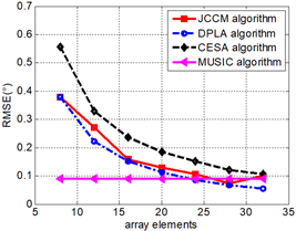
Figure 4 shows the variation in the RMSEs of the four algorithms with the number of array elements, while the other parameters were configured as: element spacing = half wavelength; number of snapshots $N=500$; arrival angles = $\text{-}{{23}^{{}^\circ }},{{42}^{{}^\circ }}$; subarray spacing $\Delta \text{=0}\text{.1}$; number of M-C cycles=500; SNR = 15dB.
Figure 4. RMSE-array element number curves
As shown in Figure 4, the DPLA algorithm outperformed CESA algorithm and JCCM algorithm, regardless of the number of array elements. When there were a few array elements, the DPLA algorithm was overshadowed by the MUSIC algorithm; when there were many array elements, the performance of our algorithm surpassed that of the MUSIC algorithm. The reason for these phenomena is still the small amount of data loss in our algorithm; but the accuracy of our algorithm was in the acceptable range.
4.2 Simulation analysis based on estimation time
The algorithm efficiency can be measured by the estimation time. Figures 5 and 6 show the estimation time of the four contrastive algorithms in MATLAB simulation, in which the parameters were configured as: element spacing = half wavelength; number of array elements $\text{2}M=16$; number of snapshots $N=500$; arrival angles = $\text{-}{{23}^{{}^\circ }},{{42}^{{}^\circ }}$; subarray spacing $\Delta \text{=0}\text{.1}$; number of M-C cycles=500; SNR = 15dB.
Figure 5. Estimation time of JCCM, DPLA and CESA algorithms
Figure 6. Estimation time of MUSIC algorithm
Obviously, our algorithm spent slightly shorter time than CESA algorithm, comparable time as JCCM algorithm, and much shorter time than MUSIC algorithm in DOA estimation. Our algorithm and JCCM algorithm boast good time performance, because they only need to process the first column of the JCCM to estimate the DOA. The CESA consumed a slightly longer time, as it needs to process the elements in the first row, first column, and the diagonal of the covariance matrix. The high time consumption of MUSIC algorithm stems from the complex operations like EVD and spectral peak search.
This paper puts forward a novel DPLA algorithm for DOA estimation, and verifies its superiority over traditional algorithms through MATLAB simulation. There are two major innovations in our algorithm: First, the rotational invariance of the two subarray signals was guaranteed by the shift invariance of the two subarrays, which eliminates the effect of array aperture and improves estimation accuracy. Secondly, our algorithm rearranges the first column elements of the JCCM into the noise subspace, and thus greatly reducing the computing load. The research results have great application potential in DOA estimation tasks.
This work was partly supported by National Natural Science Foundation of China (Grant No.: 61661030, No. 61901409).
[1] Zhang, Y., Zhang, G., Wang, X. (2016). Computationally efficient DOA estimation for monostatic MIMO radar based on covariance matrix reconstruction. Electronics Letters, 53(2): 111-113. https://doi.org/10.1049/el.2016.3818
[2] Li, B., Bai, W., Zheng, G. (2018). Successive ESPRIT algorithm for joint DOA-range-polarization estimation with polarization sensitive FDA-MIMO radar. IEEE Access, 6: 36376-36382. https://doi.org/10.1109/ACCESS.2018.2844948
[3] Huang, F., Zheng, N.N. (2019). A novel frequent pattern mining algorithm for real-time radar data stream. Traitement du Signal, 36(1): 23-30. https://doi.org/10.18280/ts.360103
[4] Saucan, A.A. (2015). Student research highlight enhanced sonar bathymetry: An echo DOA tracking approach. IEEE Aerospace and Electronic Systems Magazine, 30(6): 34-36. https://doi.org/10.1109/MAES.2015.140212
[5] Saucan, A. A., Chonavel, T., Sintes, C., Le Caillec, J. M. (2015). CPHD-DOA tracking of multiple extended sonar targets in impulsive environments. IEEE Transactions on Signal Processing, 64(5): 1147-1160. https://doi.org/10.1109/TSP.2015.2504349
[6] Li, J., Wang, Y., Le Bastard, C., Wei, G., Ma, B., Sun, M., Yu, Z. (2016). Simplified high-order DOA and range estimation with linear antenna array. IEEE Communications Letters, 21(1): 76-79. https://doi.org/10.1109/LCOMM.2016.2613867
[7] Zeng, H., Ahmad, Z., Zhou, J., Wang, Q., Wang, Y. (2016). DOA estimation algorithm based on adaptive filtering in spatial domain. China Communications, 13(12): 49-58. https://doi.org/10.1109/CC.2016.7897554
[8] Yan, G., Li, G., Ning, L. (2005). Method on fast DOA estimation of moving nodes in ad-hoc network. IEEE International Symposium on Communications and Information Technology, ISCIT 2005, Beijing, pp. 1169-1172. https://doi.org/10.1109/ISCIT.2005.1567077
[9] Levanda, R., Leshem, A. (2013). Adaptive selective sidelobe canceller beamformer with applications to interference mitigation in radio astronomy. IEEE Transactions on Signal Processing, 61(20): 5063-5074. https://doi.org/10.1109/TSP.2013.2274960
[10] Schmidt, R. (1986). Multiple emitter location and signal parameter estimation. IEEE Transactions on Antennas and Propagation, 34(3): 276-280. https://doi.org/10.1109/TAP.1986.1143830
[11] Zhang, X., Chen, W., Zheng, W., Xia, Z., Wang, Y. (2018). Localization of near-field sources: A reduced-dimension MUSIC algorithm. IEEE Communications Letters, 22(7): 1422-1425. https://doi.org/10.1109/LCOMM.2018.2837049
[12] Tan, J., Nie, Z. (2018). Polarisation smoothing generalised MUSIC algorithm with PSA monostatic MIMO radar for low angle estimation. Electronics Letters, 54(8): 527-529. https://doi.org/10.1049/el.2017.4378
[13] Roy, R., Kailath, T. (1989). ESPRIT-estimation of signal parameters via rotational invariance techniques. IEEE Transactions on acoustics, speech, and signal processing, 37(7): 984-995. https://doi.org/10.1109/29.32276
[14] Qian, C. (2018). A simple modification of ESPRIT. IEEE Signal Processing Letters, 25(8): 1256-1260. https://doi.org/10.1109/LSP.2018.2851385
[15] Bressner, T.A.H., Johannsen, U., Smolders, A.B. (2017). Single shot DOA estimation for large-array base station systems in multi-user environments. Loughborough Antennas & Propagation Conference (LAPC 2017), UK, pp. 1-4. https://doi.org/10.1049/cp.2017.0288
[16] Tian, X., Lei, J., Du, L. (2018). A generalized 2-D DOA estimation method based on low-rank matrix reconstruction. IEEE Access, 6: 17407-17414. https://doi.org/10.1109/ACCESS.2018.2820165
[17] Nie, X., Li, L. (2014). A computationally efficient subspace algorithm for 2-D DOA estimation with L-shaped array. IEEE Signal Processing Letters, 21(8): 971-974. https://doi.org/10.1109/LSP.2014.2321791
[18] Yan, F.G., Rong, J.J., Liu, S., Shen, Y., Jin, M. (2018). Joint cross-covariance matrix based fast direction of arrival estimation. Systems Engineering and Electronics, 40(4): 733-738. https://doi.org/10.3969/j.issn.1001-506X.2018.04.03
[19] Dhope, T.S., Šimunić, D., Dhokariya, N.S., Pawar, V.S., Gupta, B. (2014). What about spectrum opportunities in ‘angle’ dimension for dynamic spectrum access in cognitive radio network context? A new paradigm in spectrum sensing. Wireless Personal Communications, 76(3): 379-397. https://doi.org/10.1007/s11277-014-1712-4
[20] Palanisamy, P., Kalyanasundaram, N., Swetha, P. M. (2012). Two-dimensional DOA estimation of coherent signals using acoustic vector sensor array. Signal Processing, 92(1): 19-28. https://doi.org/10.1016/j.sigpro.2011.05.021
[21] Ingle, V.K., Proakis, J.G. (2016). Digital signal processing using MATLAB: A problem solving companion. Cengage Learning.
[22] Zhang, X.D. (2017). Matrix Analysis and Applications. Cambridge University Press.
[23] Jing, X., Du, Z.C. (2012). An improved fast Root-MUSIC algorithm for DOA estimation. 2012 International Conference on Image Analysis and Signal Processing, Hangzhou, pp. 1-3. https://doi.org/10.1109/IASP.2012.6425035