Yue Wang
© 2020 IIETA. This article is published by IIETA and is licensed under the CC BY 4.0 license (http://creativecommons.org/licenses/by/4.0/).
OPEN ACCESS
Vehicle detection and tracking are key aspects of intelligent transportation. However, the accuracy of traditional methods for vehicle detection and tracking is severely suppressed by the complexity of road conditions, occlusion, and illumination changes. To solve the problem, this paper initializes the background model based on multiple frames with a fixed interval, and then establishes a moving vehicle detection algorithm based on trust interval. The established algorithm can easily evaluate the background complexity based on regional information. After that, the authors pointed out that the correlation filtering, a classical vehicle tracking algorithm, cannot adapt to the scale changes of vehicles, due to the weak dependence of background information. Hence, a tracking algorithm that adapts to vehicle scale was designed based on background information. Finally, the proposed algorithms were proved feasible for detection and tracking moving vehicles in complex environments. The research provides a good reference for the application of computer vision in moving target detection.
video sequence, vehicle tracking algorithm, vehicle detection algorithm, intelligent transportation
Intelligent transportation [1] improves the information sharing among drivers, vehicles, and roads through the integration of various techniques, ranging from sensing, information storage, data transmission, to computer control. Intelligent transportation systems fully utilize traffic infrastructure to monitor road conditions and identify traffic events, making traffic management more intelligent.
Vehicle detection and tracking are key aspects of intelligent transportation. The vehicles could be detected and tracked by sensors and video monitors. Compared with sensors, video monitors are simple and easy to update, and capable of capturing complete information [2-4]. The traffic videos can be processed by computer vision and pattern recognition, providing effective solutions for traffic control and planning.
The detection and tracking of vehicles are critical to various traffic scenarios. In road management, the foreground objects are detected to judge whether the vehicles run the red light or enter the forbidden area. In intersection monitoring, vehicle trajectories are used to determine if the derivers violate the safety regulations. In safety management, the vehicle positions are monitored automatically in real time, reducing the hidden hazards of traffic safety. In rush hours, traffic videos help to analyze the laws of traffic flow, laying the basis for reasonable route planning.
The accuracy of vehicle detection and tracking is severely suppressed by the complexity of road conditions, occlusion, and illumination changes. It is necessary to improve the detection and tracking of vehicles based on traffic videos. Therefore, this paper fully reviews the relevant studies on moving vehicle detection and tracking. On this basis, a moving vehicle detection algorithm was developed based on trust interval, and a moving vehicle tracking algorithm was designed based on correlation filtering. The effectiveness of the algorithms was confirmed through contrastive experiments.
2.1 Moving vehicle detection methods
Moving vehicle detection aims to extract the complete contours of the moving vehicle by distinguishing between the static background and moving foreground on the road and removing the information irrelevant to the moving vehicle (i.e. noises). Currently, the common methods for vehicle detection are generally based on video sequence [5] or feature learning [6].
The video sequence-based methods can be divided into optical flow method [7], frame difference method [8], and background subtraction method [9]. The optical flow method detects moving vehicles based on the optimal flow in the video sequence. Yuan et al. [10] combined sparse optical flow and local maximum into a vehicle detection method. The frame difference method constructs the vehicle based on the pixels whose inter-frame difference surpasses the threshold. The background subtraction method detects vehicles by the difference between the current frame and the background model. The key to background subtraction lies in the background model. Wang et al. [11] proposed the Gaussian scale mixture (GSM) model based on Gaussian distribution probability. Huang et al. [12] designed the vibe model under the random strategy.
The feature learning-based methods acquires the position and contours of the vehicle in three steps: training the vehicle features in whole or in part, sliding over each frame with a fixed size window, and judging whether a part is the vehicle or background. Shiue et al. [13] described vehicles with fixed features, and developed a detection model with invariant features. Baek et al. [14] trained the detection model with adaptive boosting (AdaBoost) algorithm, and detected moving vehicles in the binary graph.
2.2 Vehicle tracking methods
In general, vehicle tracking algorithms predict the vehicle position in the next frames according to the position in the previous frames. The bases of the existing vehicle tracking algorithms include Kalman filter [15], mean shift [16], particle filter [17], and tracking learning detection (TLD) [18].
With the aid of Kalman filter, Choi et al. [19] predicted the driving state of vehicles, and matched and tracked vehicles by edge features. Li et al. [20] tracked vehicles through feature fusion and mean shift, and introduced scale-invariant feature transform (SIFT) to enhance the robustness of the tracking method. Li’s method cannot determine vehicle positions accurately, when the vehicles are blocked or cornered (i.e. the number of feature points are severely limited). Wu et al. [21] tracked vehicles based on particle filter algorithm, resampled particles with mean shift, and achieved fast convergence in local areas. Kalal et al. [22] presented a single-tracking long-term TLD algorithm, which combines tracking and detection to overcome deformation, partial occlusion, and other problems in the tracking process.
2.3 Traffic safety strategies
Vehicle detection and tracking have given rise to a series of strategies for traffic safety [23-25]. For example, Chaudhary et al. [26] counted the number of vehicles based on inter-frame difference, computed the number of moving pixels along the road in the difference binary image, and derived the traffic flow from the number and ratio of moving pixels. Ramya and Rajeswari [27] relied on frame difference and background subtraction to detect moving vehicles, tracked vehicles in virtual coils, and counted the number of vehicles. Peng et al. [28] put forward a statistical method of traffic flow, which counts the number of times that vehicles are overlapped in a fixed window based on the binary image. Zhu et al. [29] extended the support vector machine (SVM) into a detection method for abnormal vehicle behaviors: the vehicle trajectory was mapped to the vector of high-dimensional space, the sample trajectory was learned by the SVM, and then a detection model was established to detect the abnormal trajectories.
3.1 Traditional moving vehicle detection algorithms
3.1.1 Frame difference method
The grayscale of pixels is an intuitive information of videos. For two consecutive frames, the grayscale difference between pixels at the same position is positively correlated with the information change between the two frames. This correlation is adopted by the frame difference method to distinguish between two or more frames by the time axis, remove static or slowly-moving vehicles, and segment the fast-moving vehicles from the background.
If there is no moving target in the video, the grayscale of frames will remain constant, and the inter-frame difference will be zero. If there is any moving target in the video, the grayscale of the frames will change, and the inter-frame difference will be nonzero. The area of the moving target can be obtained through thresholding and morphological processing.
Let Ij(x,y) and Ij-1(x,y) be the j-th and j-1-th frames of the video sequence, respectively. The difference D(x,y) between the two adjacent frames can be defined as:
$D(x, y)=\left\{\begin{array}{ll}
1, & \left|I_{j}(x, y)-I_{j-1}(x, y)\right|>T \\
0, & \text { other }
\end{array}\right.$ (1)
where, T is a fixed threshold used to judge if pixel (x,y) belongs to the foreground. If the grayscale of the pixel is below the threshold, the pixel is a background point; otherwise, the pixel is a foreground point.
The frame difference method is a simple way to detect moving vehicles. The time interval is small between adjacent frames, and the detection is not greatly affected by illumination changes. However, this method also faces some defects, as the pixels in some areas of adjacent frames have similar grayscales. Differential processing might create holes in the adjacent frames. If the vehicle moves slowly, the target areas will overlap through differential processing. In this case, the moving vehicle will be mistaken as part of the background. If the vehicle moves rapidly, no overlap will occur after differential processing, making it impossible to separate the target region.
3.1.2 Background subtraction method
Background subtraction method, a special version of frame difference method, consists of the following steps: creating a background model based on the pixels of N consecutive frames in the video sequence; performing a differential operation between the current frame and the background; segmenting and extracting moving vehicles through thresholding and morphological operation on the processed frames. Mathematically, this method can be defined as:
$D(x, y)=\left\{\begin{array}{ll}
1, & \left|I_{j}(x, y)-B_{j-1}(x, y)\right|>T \\
0, & \text { other }
\end{array}\right.$ (2)
where, D(x,y) and B(x,y) are the j-th frame and background, respectively; T is the same as that in formula (1).
In real-world scenarios, the background changes dynamically with the surroundings. To improve the detection effect, the background must be updated constantly by:
$B_{j+1}(x, y)=(1-\beta) B_{j}(x, y)+\beta I_{j}(x, y)$ (3)
where, Bj(x,y) is the background; Ij(x,y) is the current frame; β is the background update rate.
3.2 Vehicle detection based on multi-frame interval
The traditional vehicle detection methods perform poorly in detecting moving vehicles in complex environments. To improve the performance, this paper models the initial background based on multi-frame interval, and uses to model to acquire the background samples of slowly-moving vehicles or those remaining in the scene for a short period only.
The background complexity is usually measured by how complex are the structure and color in the background. The update rate needs to be calculated constantly, and the threshold always change. In the actual scene, the threshold changes very quickly. Moreover, it is very time-consuming and compute-intensive to update the threshold and background learning rate for each frame.
To solve the above problems, a trust interval was set to judge if the current background model is suitable to update under the current traffic conditions. The interval was generated by the pixel-based adaptive segmentation algorithm [30], which automatically updates threshold R(x,y) and learning rate T(x,y) with the dynamic changes of the background. The background model B(x,y) can be defined as:
$B(x, y)=\left\{b_{1}(x, y), \cdots, b_{i}(x, y), \cdots, b_{M}(x, y)\right\}$ (4)
In the above model, the background sample is matched, if the Euclidean distance between the value I(x,y) of pixel (x,y) in the current frame and the background sample is below the threshold R(x,y). If the number of matched samples surpasses the minimum threshold Tmin, the pixel must belong to the background.
The judgement rule for foreground pixel can be defined as:
$\begin{array}{l}
D(x, y) \\
=\left\{\begin{array}{ll}
1 & \operatorname{num}\{\operatorname{dist}(I(x, y), B(x, y))<R(x, y)\}<T_{\min } \\
0 & \text { else }
\end{array}\right.
\end{array}$ (5)
where, dist(×) is the Euclidean distance between the pixel value the current position and the background sample; num(×) is the number of background samples whose Euclidean distance is below the threshold; $T_{m i n}$ is a fixed global parameter, i.e. the minimum number of matched samples. If D(x,y)=1, then pixel (x,y) belongs to the foreground.
The background of pixel (x,y) was updated as follows: If the pixel is identified as a background pixel of the current frame, then several samples were randomly selected from the background model B(x,y), and the pixel value I(x,y) was replaced with the probability of p=1/T(x,y), where T(x,y) is the learning rate.
The background of the neighbors of pixel (x,y) was updated as follows: First, a pixel (x’, y’) was selected from the neighborhood $((x, y) \in N(x, y))$ of pixel (x,y); Then, any sample in the background model B(x’, y’) of (x’, y’) was replaced by the value of pixel (x’, y’) at the probability of p=1/T(xi).
The background complexity was measured by the mean minimum distance between pixels (x,y) in the latest M frames and the background samples:
$\bar{d}_{\min }(x, y)=1 / M \sum_{j} L_{j}(x, y)$ (6)
where, Lj(x,y) is the minimum distance between the current pixel Ij(x,y) and the background sample B(x,y). If the background is very complex, the threshold R(x,y) should be large, so that background pixels will not be attributed to the foreground; if the background is not complex, the R(x,y) should be small, so that foreground pixels will not be recognized as background ones.
In addition, the learning rate T(x,y) was adaptively controlled to prevent the background model from fast integration into the background in the update process. If the current pixel belongs to the background, the learning rate will be increased; if the current pixel belongs to the foreground, the learning rate will be decreased. The adaptive control of T(x,y) can be explained as:
$T(x, y)\left\{\begin{array}{cl}
T\left(x_{i}\right)+\frac{T_{i}}{\bar{d}_{\min }(x, y)} & D\left(x_{i}\right)=1 \\
T(x, y)-\frac{T_{d}}{\bar{d}_{\min }(x, y)} & D(x, y)=0
\end{array}\right.$ (7)
where, Ti and Td are fixed increase and decrease parameters, respectively. The two parameters set the upper and lower limits for T(xi) (Tlower<T<Tupper), such that the learning rate will not exceed a certain range.
The pixel-based adaptive segmentation algorithm is a background modeler that update background models probabilistically with an adaptive threshold R(x,y) and a learning rate T(x,y). The algorithm can effectively detect moving targets in complex scenes. However, the real-time performance of the algorithm is poor, due to its heavy computing load and long computing time.
In pixel-based adaptive segmentation algorithm, the background model is initialized based on multiple continuous frames. The initialization strategy alleviates distortion, which is common in non-parametric background models based on sample points. However, the initial background model will also be distorted, if the vehicle moves slowly or remains in the scene for a short while. To optimize the background sample, multiple discontinuous images have been used to initialize the background model. The parameters should be calculated and updated in real time, and the threshold R(x,y) may increase or decrease. In the actual scene, R(x,y) is relatively stable in a short period. Based on recent traffic conditions, this paper sets a self-adjusting trust interval for the background model of each pixel. The trust interval was quantified as a value. The greater the value, the more relaxed the update requirement. Whether a background model should be updated depends on the trust interval and the recent traffic conditions.
Furthermore, the pixel-based adaptive segmentation algorithm evaluates the background complexity, without considering regional complexity. If the background is complex and the background and foreground alternate too fast, the threshold and learning rate cannot be updated in a timely and effective manner. To solve the problem, this paper evaluates background complexity based on how complex are the structure and color in the background. The evaluation result was relied on to decide whether to update the threshold and the learning rate.
Our moving target detection algorithm based on trust interval involves the following steps:
Step 1. Initialization of background model
Since the vehicle may move slowly or remain in the scene for a short period only, the background model was initialized based on multiple discontinuous frames. For pixel (x,y), the background model B’(x,y) can be initialized based on multiple frames with a fixed time interval j:
$\begin{array}{l}
B^{\prime}(x, y) \\
=\left\{b_{1}(x, y), b_{2}(x, y), \cdots, b_{i}(x, y), \cdots, b_{M}(x, y)\right\} \\
=\left\{\begin{array}{c}
I_{1}(x, y), I_{1+j}(x, y), \cdots, I_{1+(i-1) \times j}(x, y), \\
\cdots, I_{1+(i-1) \times j}(x, y)
\end{array}\right\}
\end{array}$ (8)
where, I1 is the pixel value of the first frame; I1+(M-1)´j is the pixel value of frame 1+(M-1)´j. The pixel value of the first frame was initialized as the first sample of the background model, while the pixel value of the frame 1+(M-1)´j was initialized to sample N of the background model.
Step 2. Traffic assessment and trust update
After initializing the ideal background model, the trust time period c(x,y) was set for any pixel (x,y), and referred to as the trust interval of this pixel. During this interval, the pixel is stable, and its background model needs no update. The stability and reliability of the background model are negatively correlated with the value of parameter h(x,y), i.e. the number of alternations between the foreground and background in the trust interval. If the parameter is large, the background is very unstable, calling for the update of the background model.
Similarly, the traffic state was evaluated by the trust interval. The current traffic state was divided into five levels based on the detection ratio $[e(x . y) / n(x . y)] \in[0,1]$: strongly smooth, slightly smooth, slightly blocked, moderately blocked, and strongly blocked. Note that e(x,y) is the number of times that pixels are detected as foreground in the trust interval until the end of detection, and n(x,y) is the number of frames failing in the trust interval. The state r(x,y) of the current traffic scene can be classified by:
$r(x, y)=$
$\left\{\begin{array}{l}0 \text { if }(e(x, y) / n(x, y) \leq 0.2) \text { strongly smooth } \\ 1 \text { if }\left(0.2 \leq \frac{e(x, y)}{n(x, y)} \leq 0.4\right) \text { slightly smooth } \\ 2 \text { if }(0.4 \leq e(x, y) / n(x, y) \leq 0.6) \text { slightly blocked } \\ 3 \text { if }\left(0.6 \leq \frac{e(x, y)}{n(x, y)} \leq 0.8\right) \text { moderately blocked } \\ 4 \text { if }(0.8 \leq e(x, y) / n(x, y) \leq 1) \text { strongly blocked }\end{array}\right.$ (9)
At the end of each trust interval, the value of c(x,y) was updated according to the current traffic state and pixel stability. If e(x,y)/n(x,y)<td (td is the threshold), then the background model is stable, and the background model of the current frame should be retained. In this case, the trust interval should be updated by:
$c(x, y)=\left\{\begin{array}{c}
\min (c(x, y)+10, \max c(x, y)) \\
i f(r(x, y)=0) \\
\min (c(x, y)+0, \max c(x, y)) \\
i f(r(x, y)=1 \text { or } r(x, y)=2) \\
\min (c(x, y)-1, \max c(x, y)) \\
i f(r(x, y)=3 \operatorname{or} r(x, y)=4)
\end{array}\right.$ (10)
On the contrary, if e(x,y)/n(x,y)≥td, the background model may be unstable, and the current background model should be updated to suit the dynamic conditions. In this case, the trust interval should be updated by:
$c(x, y)=\left\{\begin{array}{c}
\max (c(x, y)-10, \min c(x, y)) \\
i f(r(x, y)=0 \text { or } 4) \\
\max (c(x, y)-5, \min c(x, y)) \\
\text { if }(r(x, y)=1 \text { or } 2 \text { or } 3)
\end{array}\right.$ (11)
After classifying the input pixels, the background model was updated, in view of the changes in the background (e.g. illumination, and shadow) and moving objects (e.g. trees, slowly moving vehicles, and temporarily parked vehicles).
If the trust interval is minimized, the traffic flow at the pixel position is suitable, and the background model should be updated with the value of the potentially foreground pixel; otherwise, the model should not be updated. The selection of update method varies in different cases:
If n(x,y)<c(x,y), the background model should be updated when the following conditions are met at the same time: the current pixel is in the trust interval, the background model only suits the current traffic state r(x,y)=0, the update cycle is completed, and the current pixel I(x,y) is detected in the background. The update cycle is a fixed repetitive period for the model. Suppose the update cycle lasts 9 frames. It is judged at the 9-th frame whether the current traffic state is suitable for the update. The background model should be updated, if the said conditions are satisfied simultaneously.
If n(x,y)=c(x,y), the pixel of the current frame is at the end of the trust interval. However, the background model should still be updated, if h(x,y)/n(x,y)<td, and if the current traffic state r(x,y)=0, 1 or 2. Note that h(x,y) stores the number of alternations between foreground and background of the pixel in the trust interval.
If h(x,y)/n(x,y)<td, the traffic state is r(x,y)=0, and the pixel is stable. In this case, it is highly necessary to update the background model with the current traffic state. If h(x,y)/n(x,y)<td, the traffic state is r(x,y)=1 or 2. Since the current background is relatively stable, the background model is unlikely to be contaminated. If h(x,y)/n(x,y)≥td, the pixel is unstable, and the traffic assessment is not reliable. Thus, the background model should be updated only when the traffic state r(x,y)=0. If r(x,y)>2, it is unwise to update the background model, regardless of the value of h(x,y)/n(x,y). Otherwise, there will be a high risk of distortion.
Vehicle tracking is a basic technique in computer vision. It is the basis of advanced visual analyses, such as vehicle recognition and driving behavior analysis. The basic idea of vehicle tracking is to search the target vehicle in the neighborhood, where the target vehicle appears the previous frame. The stability of the extracted vehicle is matched with the features of the surroundings. Then, the vehicle position in the frame is detected. However, the tracking accuracy is greatly reduced by interferences, namely, occlusion, scale changes, and attitude changes during movement.
For the accuracy of vehicle tracking, this paper introduces correlation filtering to the tracking process. Correlation measures the similarity between two digital signals p and q:
$(p \otimes q)(\tau)=\int_{-\infty}^{+\infty} p^{*}(t) q(t+\tau) d t$ (12)
where, $\otimes$ is the convolution operation; p* is the complex conjugate transform of p. The correlation is positively corelated with the similarity between the two signals. Then, a filter template h was formulated. When the template convolves with the tracking object, the output response q is the largest:
$q=p \otimes h$ (13)
Kernelized correlation filter (KCF) is a highly accurate target tracking algorithm [31], which works as fast as correlation filtering in tracking moving targets. The excellence of the KCF stems from three aspects: the introduction of kernel functions into the classifier, the numerous positive and negative training samples obtained through the cyclic shift of the pixel matrix of the base image, and the training of the classifier with these samples. According to the features of the cyclic matrix, moving vehicle tracking problem is transformed into the frequency domain by Fourier transform, eliminating the need to invert the image matrix. The transform reduces the time complexity while retaining the tracking speed.
In the KCF algorithm, a classifier is trained with thousands of negative samples in each frame to improve the tracking accuracy. Meanwhile, the image block is obtained as a negative sample through cyclic shift of the base image. Then, the positive sample and the negative sample constitute a cyclic matrix for training, which ensures the real-time performance of the algorithm.
Let x=[x1, x2,…, xn]T be an $n \times 1$ vector representing the appearance of the target image block. The vector is known as the base sample (positive sample). The base sample and its various transformed versions (negative samples) are used to train the classifier. The base sample can be transformed through 1D transform of the permutation matrix vector:
$A=\left[\begin{array}{ccccc}
0 & 0 & 0 & \cdots & 1 \\
1 & 0 & 0 & \dots & 0 \\
0 & 1 & 0 & \dots & 0 \\
\vdots & \vdots & \vdots & \ddots & \vdots \\
0 & 0 & \cdots & 1 & 0
\end{array}\right]$ (14)
The matrix Ax=[xn, x1, x2,…, xn-1]τ makes the vector x shift downward by one element, mimicking a vector transform. Let Pnx be the indicator that vector x has moved u times. If u is negative, the vector is shifted in the opposite direction.
Drawing on the features of cyclic shift, signal x will be transformed into the same signal every n shifts. The complete set of shifted signals can be described as:
$\left\{A^{u} x | u=0, \dots, n-1\right\}$ (15)
Taking formula (15) as a row, the regression value of the offset sample can be computed as:
$X=C(x)=\left[\begin{array}{ccccc}
x_{1} & x_{2} & x_{3} & \cdots & x_{n} \\
x_{n} & x_{1} & x_{2} & \dots & x_{n-1} \\
x_{n-1} & x_{n} & x_{1} & \dots & x_{n-2} \\
\vdots & \vdots & \vdots & \ddots & \vdots \\
x_{2} & x_{3} & x_{4} & \dots & x_{1}
\end{array}\right]$ (16)
The resulting matrix X is a cyclic matrix, which depends on element x of the first row. The elements in the other rows are all cyclic offsets of element x. Each cyclic matrix can be described as a diagonal matrix composed of the first row of base samples x through discrete Fourier transform (DFT):
$X=\operatorname{Tdiag}(\hat{x}) T^{H}$ (17)
where, T is the constant matrix of the DFT; $\hat{x}$ is the vector x for the DFT transformation. In this paper, $\hat{x}=\mathcal{F}(x)$ represents the DFT of variables.
To detect the tracking target, the regression values of r(z) on several image blocks, which were obtained through cyclic shift, were calculated. Let Kz be the kernel correlation matrix between training samples and predicted image blocks. The samples are derived from the base sample x through cyclic shift, while the blocks are derived from image block z through cyclic shift. Therefore, any element in Kz can be obtained from κ(Pi-1z, Pj-1x). The kernel correlation matrix Kz can be expressed as:
$K^{z}=C\left(K^{x z}\right)$ (18)
where, Kxz is the kernel correlation between vectors x and z.
The regression function of all estimated image blocks z can be defined as:
$r(z)=\left(K^{z}\right)^{T} \alpha$ (19)
where, r(z) is the detection response to the image block. Each value indicates the probability that the corresponding area is the local area of the target. The maximum response corresponds to the exact position of the target. To speed up the computing, formula (19) was diagonalized by $K^{z}=\operatorname{Tgiag}\left(\hat{k}^{x z}\right) T^{H}:$
$r(\hat{z}) \hat{k}^{x z} \odot \hat{\alpha}$ (20)
Formula (29) shows that the tracking algorithm is updated in two parts: coefficient α and the target appearance model x. The update strategies of x and α are as follows:
$\alpha_{t}=(1-\beta) \alpha_{t-1}+\beta \alpha_{t}^{\prime}$ (21)
$x_{t}=(1-\beta) x_{t-1}+\beta x_{t}^{\prime}$ (22)
where, β is the learning rate; αt and αt-1 are the update coefficients of the current frame classifier and the previous frame classifier, respectively; α’t is the update coefficients of the current frame; xt and xt-1 are the update coefficients of the target appearance model of the current frame and the previous frame, respectively; x’t is the appearance model of the target in the current frame.
To evaluate its performance, the proposed algorithms were tested on several traffic video sequences under different environments. The histogram of oriented gradients (HOG) was adopted, with the cell size of 4, and the number of statistical gradient directions of 9. The target position of the initial frame was manually selected. Our algorithms were compared with popular vehicle tracking methods, namely, the KCF, circulant structure kernel (CSK), and compressive tracking (CT).
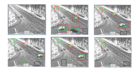
Three representative video sequences were selected from experimental video sequences to demonstrate the results of our algorithms and those of the three contrastive methods. These sequences contain challenging factors like illumination changes, motion blur, scale changes, and occlusion. The tracking results of the contrastive methods are compared in Figure 1, where the results of our algorithms are in green boxes, those of the KCF in red boxes, those of the CSK in blue boxes, and those of the CT in black boxes.
Figure 1. The tracking results of different algorithms
From frame 38 to frame 252, the vehicle motion was basically stable. All algorithms successfully positioned and tracked the vehicle. From frame 253 to frame 698, the vehicle sped up and the illumination changed greatly. In this case, the CSK and CT could not predict vehicle position accurately. Their predicted positions gradually deviated from the actual position, and eventually led to tacking failure. From frame 699 to frame 899, the vehicle scale changed constantly, while the illumination grew weaker. The vehicle motion became increasingly blurry. The KCF failed to keep track of the vehicle. Despite the changes in illumination and scale, our algorithms predicted the vehicle position accurately based on the relationship between the target and the background. This is because our position classifier grounded on the images of the vehicle and the background. The above results show that our algorithms outshine the other popular methods in robustness and accuracy, while meeting the requirement on frame rate.
This paper fully analyzes the traditional methods for moving vehicle detection, and proposes a moving vehicle detection algorithm based on trust interval. Firstly, the ideal background model was initialized based on multiple frames with a fixed interval. The background complexity was evaluated based on the complexity of structure and color. Next, a tracking algorithm that adapts to vehicle scale was extended from the KCF algorithm based on background information, aiming to enhance the dependence of correlation filtering on background information. Experimental results show that our methods can track vehicle positions accurately, and adapt to the changing scale of vehicles in complex environment.
[1] Zhang, J., Wang, F.Y., Wang, K., Lin, W.H., Xu, X., Chen, C. (2011). Data-driven intelligent transportation systems: A survey. IEEE Transactions on Intelligent Transportation Systems, 12(4): 1624-1639. https://doi.org/10.1109/TITS.2011.2158001
[2] Jazayeri, A., Cai, H., Zheng, J.Y., Tuceryan, M. (2011). Vehicle detection and tracking in car video based on motion model. IEEE Transactions on Intelligent Transportation Systems, 12(2): 583-595. https://doi.org/10.1109/TITS.2011.2113340
[3] HimaBindu, G., Anuradha, C., Chandra Murty, P.S.R. (2019). Assessment of combined shape, color and textural features for video duplication. Traitement du Signal, 36(2): 193-199. https://doi.org/10.18280/ts.360210
[4] You, F., Zhang, R., Wen, H., Xu, J. (2012). An algorithm for moving vehicle detection and tracking based on adaptive background modeling. Journal of Theoretical & Applied Information Technology, 45(2): 480-485.
[5] Zheng, F., Shao, L., Han, J. (2018). Robust and Long-Term Object Tracking with an Application to Vehicles. IEEE Transactions on Intelligent Transportation Systems, 19(10): 3387-3399. https://doi.org/10.1109/TITS.2017.2749981
[6] Tang, T., Zhou, S., Deng, Z., Zou, H., Lei, L. (2017). Vehicle detection in aerial images based on region convolutional neural networks and hard negative example mining. Sensors, 17(2): 336. https://doi.org/10.3390/s17020336
[7] Ottlik, A., Nagel, H.H. (2008). Initialization of model-based vehicle tracking in video sequences of inner-city intersections. International Journal of Computer Vision, 80(2): 211-225. https://doi.org/10.1007/s11263-007-0112-6
[8] Ramya, P., Rajeswari, R. (2016). A modified frame difference method using correlation coefficient for background subtraction. Procedia Computer Science, 93: 478-485. https://doi.org/10.1016/j.procs.2016.07.236
[9] Chen, S., Zhang, J., Li, Y., Zhang, J. (2011). A hierarchical model incorporating segmented regions and pixel descriptors for video background subtraction. IEEE Transactions on Industrial Informatics, 8(1): 118-127. https://doi.org/10.1109/TII.2011.2173202
[10] Yuan, G.W., Gong, J., Deng, M.N., Zhou, H., Xu, D. (2014). A moving objects detection algorithm based on three-frame difference and sparse optical flow. Information Technology Journal, 13(11): 1863-1867. https://doi.org/10.3923/itj.2014.1863.1867
[11] Wang, G., Schultz, L., Qi, J. (2009). Statistical image reconstruction for muon tomography using a Gaussian scale mixture model. IEEE Transactions on Nuclear Science, 56(4): 2480-2486. https://doi.org/10.1109/TNS.2009.2023518
[12] Huang, W., Liu, L., Yue, C., Li, H. (2015). The moving target detection algorithm based on the improved visual background extraction. Infrared Physics & Technology, 71: 518-525. https://doi.org/10.1016/j.infrared.2015.06.011
[13] Shiue, Y.C., Lo, S.H., Tian, Y.C., Lin, C.W. (2017). Image retrieval using a scale-invariant feature transform bag-of-features model with salient object detection. International Journal of Applied Systemic Studies, 7(1-3): 92-116. https://doi.org/10.1504/IJASS.2017.088903
[14] Baek, Y.M., Kim, W.Y. (2014). Forward vehicle detection using cluster-based AdaBoost. Optical Engineering, 53(10): 102103. https://doi.org/10.1117/1.OE.53.10.102103
[15] Yin, S. (2019). Estimation of rotor position in brushless direct current motor by memory attenuated extended Kalman filter, European Journal of Electrical Engineering, 21(1): 35-42. https://doi.org/10.18280/ejee.210106
[16] Ha, D.B., Zhu, G.X., Zhao, G.Z. (2010). Vehicle tracking method based on corner feature and mean-shift. Computer Engineering, 36(06): 196-197.
[17] Cao, X., Gao, C., Lan, J., Yuan, Y., Yan, P. (2014). Ego motion guided particle filter for vehicle tracking in airborne videos. Neurocomputing, 124: 168-177. https://doi.org/10.1016/j.neucom.2013.07.014
[18] Oh, J., Min, J., Choi, E. (2010). Development of a vehicle image-tracking system based on a long-distance detection algorithm. Canadian Journal of Civil Engineering, 37(11): 1395-1405. https://doi.org/10.1139/L10-064
[19] Choi, I.H., Pak, J.M., Ahn, C.K., Mo, Y.H., Lim, M.T., Song, M.K. (2015). New preceding vehicle tracking algorithm based on optimal unbiased finite memory filter. Measurement, 73: 262-274. https://doi.org/10.1016/j.measurement.2015.04.015
[20] Li, Z., He, S., Hashem, M. (2015). Robust object tracking via multi-feature adaptive fusion based on stability: contrast analysis. The Visual Computer, 31(10): 1319-1337. https://doi.org/10.1007/s00371-014-1014-6
[21] Wu, S.Y., Liao, G.S., Yang, Z.W., Li, C.C. (2010). Improved track-before-detect algorithm based on particle filter. Control and Decision, 25(12): 1843-1847.
[22] Kalal, Z., Mikolajczyk, K., Matas, J. (2011). Tracking-learning-detection. IEEE Transactions on Pattern Analysis and Machine Intelligence, 34(7): 1409-1422. https://doi.org/10.1109/TPAMI.2011.239
[23] Kravchenko, P., Plotnikov, A., Oleshchenko, E. (2018). Digital modeling of traffic safety management systems. Transportation Research Procedia, 36: 364-372. https://doi.org/10.1016/j.trpro.2018.12.109
[24] Pan, J., Fu, Z., Chen, H.W. (2019). A tabu search algorithm for the discrete split delivery vechicle routing problem. Journal Européen des Systèmes Automatisés, 52(1): 97-105. https://doi.org/10.18280/jesa.520113
[25] Sakhapov, R., Nikolaeva, R. (2018). Traffic safety system management. Transportation Research Procedia, 36: 676-681. https://doi.org/10.1016/j.trpro.2018.12.126
[26] Chaudhary, S., Indu, S., Chaudhury, S. (2017). Video-based road traffic monitoring and prediction using dynamic Bayesian networks. IET Intelligent Transport Systems, 12(3): 169-176. https://doi.org/10.1049/iet-its.2016.0336
[27] Ramya, P., Rajeswari, R. (2016). A modified frame difference method using correlation coefficient for background subtraction. Procedia Computer Science, 93: 478-485. https://doi.org/10.1016/j.procs.2016.07.236
[28] Peng, Y., Chen, Z., Wu, Q.J., Liu, C. (2018). Traffic flow detection and statistics via improved optical flow and connected region analysis. Signal, Image and Video Processing, 12(1): 99-105. https://doi.org/10.1007/s11760-017-1135-2
[29] Zhu, S., Hu, J., Shi, Z. (2016). Local abnormal behavior detection based on optical flow and spatio-temporal gradient. Multimedia Tools and Applications, 75(15): 9445-9459. https://doi.org/10.1007/s11042-015-3122-3
[30] Li, W., Zhang, J., Wang, Y. (2019). WePBAS: A weighted pixel-based adaptive segmenter for change detection. Sensors, 19(12): 2672. https://doi.org/10.3390/s19122672
[31] Henriques, J.F., Caseiro, R., Martins, P., Batista, J. (2014). High-speed tracking with kernelized correlation filters. IEEE Transactions on Pattern Analysis and Machine Intelligence, 37(3): 583-596. https://doi.org/10.1109/TPAMI.2014.2345390