Zaki Aissam Khezzar* | Redha Benzid | Lamir Saidi
© 2020 IIETA. This article is published by IIETA and is licensed under the CC BY 4.0 license (http://creativecommons.org/licenses/by/4.0/).
OPEN ACCESS
The presented method is a DCT mitigation thresholding technique (DCT-MTT) for narrowband interference reduction in Global Navigation Satellite System (GNSS) receivers. First, the received signal immersed in an Additive White Gaussian Noise (AWGN), is multiplied, in time domain, (sample by sample) by a Tukey window of the same length. Then, the DCT transform is applied. Next, the transformed signal is divided in non-overlapped packets. Each one can be viewed as a non-interfered packet (if it has roughly the same variance as the estimated unknown variance of the AWGN) that must be conserved, or considered as an interference packet (if its variance is significantly greater than the variance of the AWGN) that should be thresholded. The conservation (or inversely the thresholding) of a packet is achieved by the use of DONOHO’s Universal-Threshold apart from that the variance is estimated based on the statistical sampling theory. The Final step consists in the application of the inverse DCT to obtain a good approximation of the received interference-less signal. The results obtained from several simulations confirm that the suggested strategy outperforms, in term of signal quality restoration, the conventional methods.
GNSS interference mitigation, DSSS, Discrete cosine transform, Universal threshold, statistical sampling theory, Tukey window, narraw band interference (NBI)
Navigation systems play a significant role in today’s localization based services. The need to such systems is growing rapidly in several fields such as: Intelligent transport systems, Military sectors, smart phone applications, agriculture and related industry and many others. Unfortunately, the GNSS receivers are vulnerable to contamination by unintentional interferences generated by other communication systems and/or intentional interferences known also as jamming. Thus, these kind vulnerabilities can disrupt GNSS-based services in widespread geographical areas [1].
In this context, an integrated solution for interference mitigation employed at the receiver is required. As one of the most used anti-jamming strategies, the pre-correlation interference countermeasures consisting in the techniques that operate before the acquisition process. Such techniques can be classified into three classes. The first class includes antennas-based solutions. As a representative example, the work that used antenna arrays adopted to produce radiation pattern which reduces the interference signal coming from a determined direction [2]. The second group comprises front-end part solutions. As a belonging method, the Automatic Gain Control (AGC) that can be used as a helpful tool to detect and estimate the interference [3]. Additionally, the third category encompasses the digital signal processing (DSP) based solutions, which are applied at the front-end output. The DSP algorithms used for GNSS jamming mitigation can be roughly divided into two main sub-categories: temporal domain and transform domain filtering techniques. Time domain processing is the simplest way which acts directly to process contaminated data and therefore is appropriate and of low cost [4]. A detection and mitigation method for narrowband interference [5] is proposed based on an adaptive infinite impulse response (IIR) notch filter (NF) that adaptively estimates the notch frequency, where the magnitude of estimated zero of notch filter placed near to unity in the presence of CW interference and otherwise it remains close to zero. In the same context, an adaptive IIR notch filter and adaptive cascading filter structure was employed to identify the type of interference signals [6]. Also, a simple mechanism achieves pulsed interference suppression in the time domain by thresholding output samples of the ADC converter [7]. In counterpart, transform domain filtering techniques transform the altered input data in a different domain. One of the belonging methods that engaged the Discrete Fourier Transform (DFT) to mitigate the interference is reported in the study [8]. It acts by modifying the spectrum of the contaminated input data, in the Fast Fourier Transform (FFT) domain. Therefore, spectral lines of the interference are blanked (removed) from the received signal according to the determined excision threshold. Additionally, the short time Fourier transform (STFT) is used to estimate the instantaneous frequency of interference in Time-Frequency TF domain, next an IIR filter is applied as a rejector [9]. Likewise, an STFT-based interference excision system is proposed by Quyang and Amin [10]. However, due to the well-known reported drawback of the STFT method, that is the fixed length analyzing window, the wavelet transform (WT) appeared to offer more flexibility on the choice of window length (by using multi-resolution analysis). Consequently, considered as another alternative, the interference mitigation by Wavelet Packet Decomposition (WPD) filtering is introduced in the researches [11, 12]. The method employed Donoho’s de-noising thresholding principle to estimate the interference. Accordingly, the useful signal is finally obtained by subtraction of the estimated interference from the received signal. In this context, the authors [1] proposed empirical thresholds based on the standard deviation estimation of each wavelet packet in absence of the interference. Hence, the reduction of the interference is performed by the suppression of all coefficients that are above the empirically defined thresholds.
In this paper, the authors describe a transform domain method considering an innovative thresholding technique to reject narrowband interference. First, the received signal, which is assumed contaminated by an Additive White Gaussian Noise (AWGN), is multiplied, in time domain, (sample by sample) by a Tukey window of the same length. Next, it is transformed in the DCT domain. After that, the transformed signal is partitioned in non-overlapped packets. Each one can be a non-interfered packet (of the same variance of the AWGN) that should be preserved, or an interference packet (if its variance is significantly greater than the variance of the AWGN) that should be thresholded. The preservation (or conversely the thresholding) of a packet is achieved by the use of the well-established Universal-Threshold of DONOHO’s algorithm apart from that the variance is estimated based on the statistical sampling theory. The last stage consists in the application of the inverse DCT to obtain a good estimation of the AWGN.
The paper is organized as follows: Received signal model and the classification of interference signals characteristics are introduced in section 2. The mathematical background concerning the DCT Transform, the universal threshold and the statistical sampling theory are presented in the section 3. Detailed model of the interference mitigation suppression will be described in section 4. Simulation results evaluate the suppressing interference method performance will be discussed in Section 5. Finally, a conclusion section concludes the paper.
2.1 Signal modeling
The received interfered GNSS signal at the input of a front-end receiver can be expressed by:
$r\left( t \right)=\underset{i=0}{\overset{M-1}{\mathop \sum }}\,{{s}_{i}}\left( t \right)+j\left( t \right)+n\left( t \right)\,$ (1)
where, M indicates the total number of visible satellites, Si(t) denotes the transmitted GNSS signal received from the ithobservable satellite, however, j(t)is the RF corrupting interference, and n(t) is the additive white Gaussian noise (AWGN). Note that, every useful GNSS channel can be describe by [1]:
$\begin{array}{*{35}{l}} s\left( t \right)=\sqrt{2P}d\left( t-{{\tau }_{0}} \right)c\left( t-{{\tau }_{0}} \right){{s}_{c}}\left( t-{{\tau }_{0}} \right) \\ \text{cos}\left( 2\pi \left( {{f}_{E}}+{{f}_{d}} \right)t+{{\varphi }_{0}} \right) \\\end{array}$ (2)
where, P is the power of the received signal, d(t) is the navigation message component, c(t) is the spreading sequence of the captured satellite, while $\tau_{0}$, fd, and $\varphi_{0}$are, respectively, the received code delay, the Doppler frequency, and the phase produced by the channel; $f_{E}$ is the central frequency of GNSS signal
The signal in Eq. (1) is then delivered to receiver front-end passing through several steps, next, it is down-converted to the intermediate frequency (IF) and sampled at rate fs=1/Ts. Therefore, at the ADC output the composite received signal can be described as follows:
$r\left( n \right)=s\left( n{{T}_{s}} \right)+j\left( n{{T}_{s}} \right)+n\left( n{{T}_{s}} \right)$ (3)
It is worth noting that j(nTs) and n(nTs)are, respectively, the sampled interference and the digital AWGN components. Additionally, for a given front-end bandwidth $B_{\mathrm{IF}}$, it can be noticed that by sampling the signal at the Nyquist frequency fs=2BIF, the noise variance becomes [1, 13]:
$\sigma _{IF}^{2}=E\left\{ {{n}^{2}}\left[ n \right] \right\}=\frac{{{N}_{O}}~{{f}_{s}}}{2}={{N}_{O}}~{{B}_{IF}}$ (4)
where, N0 is the power spectral density (PSD) of the noise.
Note that the digitized GNSS signal from visible satellite is stated by:
$\begin{array}{*{35}{l}} s\left( n \right)=\sqrt{2P}d\left( n{{T}_{s}}-{{n}_{0}} \right)c\left( n{{T}_{s}}-{{n}_{0}} \right){{s}_{c}}\left( n{{T}_{s}}-{{n}_{0}} \right) \\ \text{cos}\left( 2\pi \left( {{f}_{E}}+{{f}_{d}} \right)n{{T}_{s}}+{{\theta }_{0}} \right) \\\end{array}$ (5)
2.2 Interference signal description
Interference usually transmits high-power signal that produces, consequently, the receiver loss when acquiring and tracking GNSS signals. Therefore, GNSS receivers can be polluted by diverse kinds of interference. The most of the Radio Frequency interference (RFI) are considered Narrowband interferences (NBI). Additionally, one of the most existing and of disastrous impact is the CWI interference which has the spectral occupation tending to zero. It can easily diminish drastically the performance of a GNSS receiver. Another type of interference, that can be faced, is the pulsed signals transmitted from Distance Measuring Equipment/Tactical Air Navigation interference DMA/TACAN services [13]. It is noted that such type shares the same spectrum of the satellite navigation systems, as well as the occupation of pulse interference is considered as a narrowband one. Accordingly, the preceding cited interferences can be modeled as follows:
(a) Single-tone continuous wave interference (SCWI)
${{j}_{scwi}}\left( t \right)=J\text{cos}\left( 2\pi \left( {{f}_{IF}}\pm \Delta f \right)t+\varnothing \right)$ (6)
where, J is the interfering signal amplitude and $\Delta f$ is the difference from the central frequency of the GNSS signal, and $\varnothing$ is a random initial phase uniformly distributed in the interval [ $-\pi, \pi$].
(b) Multi-tone continuous wave interference (MCWI)
${{j}_{mcwi}}\left( t \right)=\underset{i=1}{\overset{N}{\mathop \sum }}\,{{J}_{i}}\cos \left( 2\pi \left( {{f}_{IF}}\pm \Delta {{f}_{i}} \right)t+{{\varnothing }_{i}} \right)~$ (7)
where, Ji, $\Delta f_{i}$ and $\varnothing_{i}$ are, respectively, the amplitude, the frequency difference, and the random phase for the ith tone.
(c) Pulse interference
$\begin{align} & j\left( t \right)=\sqrt{P~}\underset{i=1}{\overset{M}{\mathop{\mathop{\sum }^{}}}}\,\left( {{e}^{\frac{-\alpha {{\left( t-{{t}_{k}} \right)}^{2}}}{2}}}+{{e}^{\frac{-\alpha {{\left( t-\text{ }\!\!\Delta\!\!\text{ }t-{{t}_{k}} \right)}^{2}}}{2}}} \right)\times \text{cos}\left( 2\pi ({{f}_{IF}}\pm \Delta f \right)t\, \\ & +\varnothing ) \\\end{align}$(8)
where, P is the DME/TACAN peak power at the antenna, tk is the set of pulse pairs arrival times, fIF is the frequency of the received interference, $\varnothing$ is the interference signal carrier phase, $\Delta t=12 \mu s$ is the inter-pulse interval and $\alpha$=4.5´1011S-2. Figure 1 shows a DME/TACAN pulse pair [14].
Figure 1. DME pulse pair signal waveform after modulation
3.1 Discrete cosine transform
The Discrete Cosine Transform (DCT) is a well-known and one of the most used transform to signal processing and analyzing in frequency domain. It is expressed by Eq. (9):
\(R\left( k \right)=w\left[ k \right]\underset{k=1}{\overset{N}{\mathop \sum }}\,r\left[ n \right]cos\frac{\pi \left( 2n-1 \right)\left( k-1 \right)}{2N}~\text{ }/k=1,\ldots \ldots ..,N\) (9)
where,
$w\left[ k \right]=\left\{ \begin{matrix} ~\frac{1}{\sqrt{N}}~~~~~~~~~~~~~~~~~k=1 \\ \sqrt{\frac{2}{N}}~~~~~~~~2\le k\le N \\\end{matrix} \right.~~$
N is the length of the time domain input signal r.
It is noticeable that the frequency index k, is formulated by [15]:
$\begin{align} & k=\left\lfloor \frac{N\times f}{fs/2} \right\rfloor \\ & f=\frac{k\times fs}{2N} \\\end{align}$
where, fs is the sampling frequency, f is the frequency corresponding to the kth index and $\lfloor.\rfloor$ is the rounding off operator to the nearest integer operator.
On the other hand, the inverse DCT is presented in Eq. (10).
$r\left( n \right)=\underset{k=1}{\overset{N}{\mathop \sum }}\,w\left[ k \right]R\left[ k \right]cos\frac{\pi \left( 2n-1 \right)\left( k-1 \right)}{2N}~$ (10)
It is worthy to note that the DCT transform is among real-to-real transforms. In fact, the DCT is a fast transform which decomposes signal to harmonics in the range $\left[0-\frac{F s}{2}\right]$ Hz.
3.2 Universal threshold
Discrete Wavelets transform DWT provides an efficient way to estimate signals in the presence of noise. The signal denoising based on DWT is constituted of three steps that are [16, 17]:
- The decomposition of the signal by means of the DWT;
- The thresholding of the wavelet coefficients that may contain mainly the noise in order to reduce the noise pollution of the useful signal;
- Finally, the reconstruction phase and the restoration of the useful signal which is achieved by the application of the inverse DWT.
Donoho and Johnstone introduced an innovative nonlinear approach for thresholding in wavelet domain. In their technique, the thresholding can be applied by implementing hard or soft thresholding strategies, which also called as shrinkage [16]. The threshold value $\lambda_{u n i v}$ of the denoising functions is based on the estimation of the noise assumed existing in the data. Hence, the universal threshold proposed by Donoho can be expressed as:
$\,{{\lambda }_{univ}}=\sigma \sqrt{2logN}$ (11)
where, N is the signal length and $\sigma$ is the standard deviation of the noise. Note that the noise level $\sigma$ was estimated by the estimator involving the calculation of the median of the absolute values of the wavelet coefficients of the first detail level [16, 17] expressed in Eq. (12):
$\,\sigma =\frac{Median\left( \left| c{{D}_{j}} \right| \right)}{0.6745}$ (12)
Consequently, the hard threshold is achieved according to Eq. (13):
$\,Hard-threshold\,\,\,\,\left\{ \begin{matrix} y=x~if~\left| x \right|>\lambda \\ y=0~if~\left| x \right|<\lambda \\\end{matrix} \right.$ (13)
However, the soft-thresholding is ensured according to Eq. (14):
$Soft-threshold\,\,\,\,\,\,\,\,\left\{ y=sign\left( x \right) \right.\left( \left| x \right|-\lambda \right)$ (14)
where, x is the input signal and y is the signal after threshold.
3.3 Standard deviation estimation using the sampling theory
In most denoising methods, reported in the literature, the well-established DONOHO’s estimator (Eq. (12)) is involved to estimate the unknown standard deviation $\sigma$ of the AWGN. However, in our contribution, the unbiased estimator deduced from the sampling theory is used [18]. It is described by:
$\sigma =\sqrt{\frac{1}{L-1}\underset{i=1}{\overset{L}{\mathop \sum }}\,{{\left( z_{i}^{2}-\mu \right)}^{2}}}$ (15)
where, $\mu$, the sample mean, is described by:
$\mu=\frac{1}{L} \sum_{i=1}^{L} z_{i}$
where, L is the length of a sample frame (packet).
3.4 The cosine-tapered window (Tukey window)
By multiplying, sample by sample, the input signal by the cosine-tapered window, the boundaries effects are considerably reduced when using the DCT-based thresholding. The mathematical model of the Tukey window is expressed as follows [19].
$w\left( x \right)=\left\{ \begin{matrix} \begin{align} & \frac{1}{2}\left\{ \left. 1+\text{cos}(\frac{2\pi }{r}\left( x-r/2 \right) \right\} \right.\text{ }(0\le x<\frac{r}{2}) \\ & 1\text{ }(0\le x<1-\frac{r}{2}) \\\end{align} \\ \frac{1}{2}\left\{ \left. 1+\text{cos}(\frac{2\pi }{r}\left( x-1+r/2 \right) \right\} \right.\,\,\,\,\,\,\,(1-\frac{r}{2}\le x<1) \\\end{matrix} \right.~$ (16)
where, r is the ratio of cosine-tapered section length to the entire window length N with 0 ≤ r ≤ 1.
4.1 Proposed mitigation thresholding technique
Inspired by the well-established Donoho’s wavelet-based thresholding technique [16, 17] used in the wavelet domain, additionally, motivated by the works presented in the researches [20, 21] that used the thresholding strategy in the DCT domain for speech enhancement, also the work estimating the AWGN standard deviation by the sampling theory estimator [18] for ultrasonic signals denoising, the proposed technique provides a new GNSS interference mitigation method in the DCT domain. Accordingly, the interference mitigation unit is incorporated in the pre-despreading part of the GNSS receiver. Figure 2 shows the different constituting blocks of the suggested method.
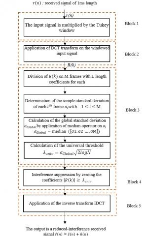
As shown, first, the incoming signal $r(n)$ is multiplied by a Tukey window in order to diminish the border effect. Then, the resulting signal is transformed in DCT domain. Next, the transformed signal is devised into adequate number of segments in order to estimate the sample standard deviation ($\sigma_{i}$ with $1 \leq i \leq \mathrm{M}$) of each $i^{t h}$ segment (packet) separately, to estimate a global standard deviation ($\sigma_{G l o b a l}$) by a suggested strategy. Then the threshold of the excision phase is determined according to the universal threshold method. Consequently, the coefficients above the calculated threshold are nullified. Finally, the application of the inverse DCT operation recovers, suitably, the received signal of reduced-interference. For more illustration of the proposed approach, a summarizing flowchart is shown in Figure 3.
Figure 2. Scheme of the proposed GNSS interference mitigation unit
Figure 3. The flow chart of the proposed interference mitigation unit
The performance of the proposed algorithm was obtained using an open-source simulator in MATLAB. Therefore, the algorithm has been simulated as user defined block integrated in the simulator [22].
5.1 The Galileo E5 signal presentation
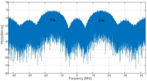
The Galileo E5 is constituted of two bands, the first one is centered at 1176.45 MHz and the second is centered at 1207.140 MHz. Accordingly, the Galileo E5 signal is an AltBOC (15,10) modulated signal with a chipping rate of 10.23 Mbps. The Figure 4 illustrates the simulated power spectral densities (PSD) of E5 band in which we observe at the receiver front end that the signal is submerged within AWGN because of its weakness like the others GNSS systems.
5.2 The open-source `GE5-TUT' Galileo simulator
This Galileo open-source simulator is dedicated to the E5 band. It is a potent manner that allows the evaluation of the performance of suggested solutions trying to solve several faced types of problems that may degrade receiver efficiency. The simulator allows simulation of data transmission, which is composed of three essential blocks that are: Transmitter, propagation channel and the receiver block [22]. Consequently, the Galileo E5a-I signal has been chosen in all our simulation scenarios.
Figure 4. Power Spectral Densities (PSD) of E5 band
Details about signal parameters are enumerated in Table 1.
Table 1. E5aI signal parameters
|
Parameters |
Value |
|
Desired signal |
Galileo E5a-I |
|
Sampling frequency fs |
31.500 MHz |
|
Intermediate frequency fIF |
4.655 MHz |
|
Coherent integration |
1ms |
|
CNR |
49 dB-Hz |
It is worthy to note, that the performance of the suggested method is evaluated in terms of:
$c=\frac{\mathop{\sum }_{i=1}^{N}\left( r-\bar{r} \right)\left( \hat{r}-\overline{{\hat{r}}} \right)}{\sqrt{\mathop{\sum }_{i=1}^{N}{{\left( r-\bar{r} \right)}^{2}}}\sqrt{\mathop{\sum }_{i=1}^{N}{{\left( \hat{r}-\overline{{\hat{r}}} \right)}^{2}}}}$ (17)
where, r is the original signal and $\hat{r}$ is the retrieved signal.
In order to demonstrate the effectiveness of the suggested DCT-MTT, two scenarios have been studied.
5.3 First scenario: continuous waves interference mitigation
The simulation test is composed of the Galileo E5aI signal and the added continuous waves interference signal. The interference to signal ration ISR of the SCWI and MCWI is between 10-60 db. It is calculated with:
$\,ISR=10log{}^{I}/{}_{S}$
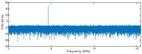
where, I is the interference power and S is the legitimate signal power, Note that the employed CWI, is a pure sinusoidal signal in the case of SCWI, located in the center of the main lobe at the intermediate frequency FI = 4.655 MHz of E5a band which corresponds to a carrier frequency of 1176.45 Mhz. This scenario presents the most dangerous attack. For more illustration, the Power Spectral Density (PSD) of the interfered signal with 50dB is presented in Figure 5.
Figure 5. PSD of the contaminated input signal E5a with ISR=50dB
At first, we investigate the anti-jamming method performance in the presence of SCWI. The jammer power is increased by means of the signal generator, so the ISR is varying from 10 to 60 dB.
It is well known that the DCT thresholding of a signal of a limited length produces a serious borders effect. To overcomes the faced problem, we found that the Tukey window (N,0,05) reduces considerably the border effect after the DCT-thresholding followed by the inverse-DCT.
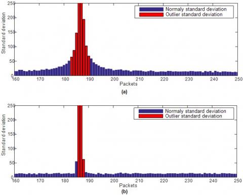
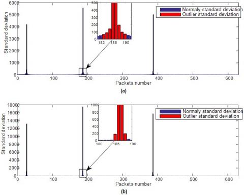
Accordingly, like wavelet thresholding strategy, in the DCT domain, the determination of a suitable threshold determination is a task converging to a successful restoration of the useful information. In order to obtain the threshold, the resulting frequency signal from the DCT transform application is divided into M non-overlapped packets of L coefficients each. We found, empirically, that the suitable length of each packet can be L=50 coefficients. Consequently, the resulting number of packets is M=630, which gives a good statistical reading of the input signal state. From the Figure 6 we notice the reduction of interfered packets due to narrowed border effect around the central interference frequency (due to the Tukey window use), accordingly, the interference position is localized accurately. It is reported that the non affected packets have roughly the same variance of the Gaussian distribution.
Once the vector of the standard deviations of all packets are obtained, the median operator is applied on the entire vector $\sigma_{i}=\left[\sigma_{1}, \cdot \sigma_{2}, \cdot \sigma_{3} \ldots, \cdot \sigma_{630}\right]$. Therefore, the interfered standard deviations (outlier packets) are rejected and the global standard deviation ($\sigma_{G l o b a l}$) is estimated. Then, the universal threshold $\lambda_{u n i v}$ is adjusted according to DONOHO’s thresholding principle.
The next operation is the threshold of the DCT coefficients. Therefore, all the coefficients surpassing $\lambda_{u n i v}$ value are nullified. The resulting modified coefficients vector leads to a good quality approximation of the interference-free signal when applying the inverse DCT.
Figure 6. Effect of the Tukey window on the standard deviations estimation, (a) the standard deviations of the interfered packets without Tukey window use, (b) the standard deviations of the interfered packets with Tukey window use
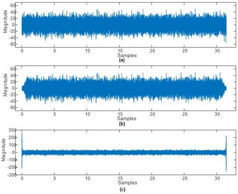
Figure 7 illustrates the time representation of the restored signal resulting from the DCT-based thresholding. It reveals that there is a substantial drop of border effect when using Tukey window. Additionally, by a visual inspection, it can be observed that the similarity between retrieved signal Figure 7(b) and the original non-contaminated signal Figure 7(a) is clear compared to the restored signal (without Tukey window) in Figure 7(c).
Following the same reasoning, we inspect the suggested anti-jamming approach performance in the presence of Multi continuous waves MCWI, where the situation is more complicated for the receiver. Thus, more interference harmonics are included in a way to contaminate more than the main lob. Consequently, multi band will be rejected. Figure 8 shows the interfered packets according to MCWI contamination, three detected bands are investigated. Interestingly, with Tukey window the interference is better localized.
Additionally, the Figure 9 illustrates the time representation of the restored signal. From Figure 9(c), it can be seen that the border effect has an important value compared to border effect of the SCWI, while in Figure 9(b), the border effect is drastically attenuated by the use of Tukey windows.
Figure 7. Restored signal after interference mitigation unit for SCWI, (a) time representation of the original non contaminated signal, (b) the restored signal (when using the Tukey windows) the restored signal presenting a significant border effect (without using the Tukey windows)
Figure 8. Enhancement reported by using the Tukey window on the standard deviations estimation with MCWI, (a) the standard deviations of the interfered packets without Tukey window use, (b) the standard deviations of the interfered packets with Tukey window use
Figure 9. Restored signal after interference mitigation unit for MCWI, (a) time representation of the original non-contaminated signal, (b) the restored signal (with Tukey windows use), (c) the restored signal showing the border effect (without using Tukey windows)
For more illustration, Figure 10 Depicts the impact of the suggested mitigation approach on the ambiguity function measure. It is apparent from Figure 10(a) that the ambiguity function obtained from the contaminated signal do not shows any dominant or secondary correlation peaks which leads, consequently, to a wrong estimation of the acquisition parameters in the presence of MCWI (50 dB). However, Figure 10(b) shows the correlation peak when the interference mitigation block is activated.
Quantitatively, the Table 2 compares the $\alpha_{\max }$ of the retrieved signal resulting from the DCT-MTT for both single and multi-interference with the corresponding one resulting from the application of the conventional IIR notch filter mitigation method [1, 22, 24].
Table 2. Acquisition metric $\alpha_{\max }$ after interference removal for MCWI and SCWI
|
Mitigation method |
Single inteference |
Multi inteference |
|
IIR notch filter |
1.93 |
1.731 |
|
Proposed DCT-based thresholding |
2.05 |
1.978 |
Figure 10. Ambiguity functions of the Galileo E5a signal in the presence of MCWI (ISR=50dB) (a) Without interference rejection unit, (b) With the proposed interference rejection unit
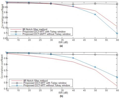
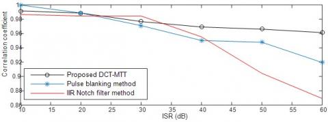
Moreover, Figure 11 confirms the effectiveness of the suggested method when using the correlation coefficient as a metric. Consequently, the compared methods to the proposed DCT-MTT using Tukey window approach are respectively: the DCT-MTT without Tukey window and the conventional IIR notch filter.
Figure 11. Comparative results using the correlation coefficient metric (a) Correlation Coefficient in the case of SCWI mitigation, (b) Correlation Coefficient resulting from MCWI mitigation
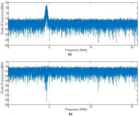
For more convincing performance evaluation, the PSDs of the contaminated and the restored signals are presented in Figure 12. It is clear, that the DCT-MTT strategy application for MCWI mitigation on the E5a Galileo signal, enhances, significantly the quality of the restored signal.
Figure 12. The PSDs of: (a) The PSD of contaminated signal (ISR=50dB), (b) the PSD of the restored signal after MCWI rejection
Second scenario: Pulse interference
As mentioned, previously, the Galileo E5a/E5b signals and others new GNSS signal suffer from interference transmitted in their band by the DMA/TACAN signals. Accordingly, to evaluate the performance and efficiency of the suggested algorithm, we simulate the Galileo E5aI infection by a pulsed signal with 3000 pulses per second. Figure 13 shows an interval of a 2ms navigation signal corrupted by a DMA signal of a pulse density of 3000 pps according to a power of 50 dB.
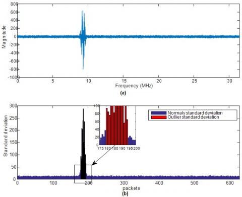
As illustrated previously by the flowchart of Figure 3 and as explained in the first scenario of continuous wave interference removing, the same strategy is adopted, however, in the DMA interference case, the Tukey window is not used. The Figure 14 represent the standard deviations estimation phase.
Figure 13. Time domain E5aI signal corrupted by a pulsed DMA signal of 3000 pps and ISR=50dB
Figure 14. The standard deviations estimation, (a) DCT represenation of the contaminated signal (b) the estimation of the standard deviations of the packets
Next, Figure 15 provides an overview of the impact of the proposed method on the ambiguity function of the Galileo E5a signal.
Additionally, the proposed DCT-MTT is compared to the pulse blanking method [7, 22] and the IIR notch filter [22] according to the $\alpha_{\max }$ metric. Table 3 presents the obtained results from the acquisition search space.
Table 3. Acquisition metric $\alpha_{\max }$ after interference removal of DMA interference
|
Pulse interference method suppression |
$\alpha_{\max }$ |
|
Proposed DCT- based thresholding |
1.86 |
|
Pulse blank method |
1.84 |
|
IIR notch filter |
1.63 |
Figure 15. Ambiguity function of the Galileo E5a signal in the presence of a pulse interference (ISR=50dB and 3000 pps), (a) Without interference rejection unit, (b) With the proposed interference rejection unit
Figure 16. Comparative results according to the correlation coefficient metric (DMA pulse interference of density of 3000 pps)
Figure 17. The PSDs, (a) the PSD of contaminated input signal, (b) the PSD of restored signal after DMA interference, of ISR=50 dB and 3000 pps, rejection
Figure 16 proffers results of the previous mentioned methods according to the correlation coefficient metric. From results, the effectiveness of DCT-MTT approach in the case of pulse scenario is demonstrated. In addition, comparison between the PSDs of received interfered signal by a DMA interference and the signal after the interference mitigation unit is shown in the Figure 17.
In this paper a DCT-MTT for NBI interference mitigation was presented. The technique proffers several advantages as a result of: The time-domain multiplying by Tukey window that reduce considerably the border effect, the fine interference localisation in the DCT-domain, the efficient threshold estimation inspired from DONOHO’s thresholding method in association of the statistical sampling theory. Comparison between the suggested strategy and conventional methods validate that our technique is of superior and concurrent performances.
[1] Musumeci, L., Curran, J.T., Dovis, F. (2016). A Comparative analysis of adaptive a notch filtering and wavelet mitigation against jammers interference. Journal of the Institute of Navigation, 63(4): 533-550. https://doi.org/10.1002/navi.167
[2] Konovaltsev, A., De Lorenzo, D.S., Hornbostel, A., Enge, P. (2008). Mitigation of continuous and pulsed radio interference with GNSS antenna arrays. Proceedings of the 21st International Technical Meeting of the Satellite Division of the Institute of Navigation (ION GNSS ’08), Savannah, Ga, USA, pp. 2786-2795.
[3] Savasta, S., Dovis, F., Lesca, R., Margaria, D., Motella, B. (2008). On the interference mitigation based on ADC parameters tuning. Proceedings of the IEEE/ION Position, Location and Navigation Symposium (PLANS ’08), pp. 689-695. https://doi.org/10.1109/PLANS.2008.4570026
[4] Mosavi, M., Shafiee, F. (2016). Narrowband interference suppression for GPS navigation using neural networks. GPS Solutions, 20(3): 341-351. https://doi.org/10.1007/s10291-015-0442-8
[5] Borio, D., Camoriano, L., Presti, L.L. (2008). Two-pole and multi-pole notch filters: A computationally effective solution for GNSS interference detection and mitigation. IEEE System Journal, 2(1): 38-47 https://doi.org/10.1109/JSYST.2007.914780
[6] Kang, C.H., Kim, S.Y., Park, C.G. (2013). A GNSS interference identification using an adaptive cascading IIR notch filter. GPS Solutions, 18(4): 605-613. https://doi.org/10.1007/s10291-013-0358-0
[7] Erlandson, R.J., Kim, T., Hegarty, C., van Dierendonck, A.J. (2004). Pulsed RFI effects on aviation operations using GPS L5. Proceedings of the National Technical Meeting of The Institute of Navigation (NTM ’04), San Diego, Calif, USA, pp. 1063-1076.
[8] Capozza, P.T., Holland, B.J., Hopkinson, T.M., Landrau, R.L. (2000). A single-chip narrow-band frequency-domain excisor for the global positioning system (GPS) receiver. IEEE Journal of Solid-State Circuits, 35(3): 401-411. http://dx.doi.org/10.1109/4.826823
[9] Borio, D., Camoriano, L., Savasta, S., Presti, L.L. (2008). Time-frequency excision for GNSS applications. IEEE Syst Journal, 2(1): 27-37. http://dx.doi.org/10.1109/JSYST.2007.914914
[10] Quyang, X., Amin, M.G. (2001). Short-time fourier transform receiver for non-stationary interference excision in direct sequence spread spectrum communications. IEEE Transactions on Signal Processing, 49(4): 851-863. https://doi.org/10.1109/78.912929
[11] Landry, R.J., Mouyon, P., Lekaim, D. (1998). Interference mitigation in spread spectrum systems by wavelet coefficients thresholding. European Transactions on Telecommunications, 9(2): 191-202. https://doi.org/10.1002/ett.4460090209
[12] Mosavi, M., Rezaei, M., Pashaian, M., Moghaddasi, M. (2018). A fast and accurate anti-jamming system based on wavelet packet transform for GPS receivers. GPS Solutions, 21(2): 415-426. https://doi.org/10.1007/s10291-016-0535-z
[13] Musumeci, L., Dovis, F. (2014). Use of the wavelet transform for interference detection and mitigation in global navigation satellite systems. International Journal of Navigation and Observation, 2014: 1-14. https://doi.org/10.1155/2014/262186
[14] Musumeci, L., Samson, J., Dovis, F. (2014). Performance assessment of pulse blanking mitigation in presence of multiple Distance Measuring Equipment/Tactical Air Navigation interference on Global Navigation Satellite Systems signals. IET Radar, Sonar & Navigation, 8(6): 647-657. https://doi.org/10.1049/iet-rsn.2013.0198
[15] Shin, H., Lee, C., Lee, M. (2010). Ideal filtering approach on DCT domain for biomedical signals: Index blocked DCT filtering method (IB-DCTFM). Journal of Medical Systems, 34(4): 741-53. https://doi.org/10.1007/s10916-009-9289-2
[16] Donoho, D.L., Johnstone, I.M. (1994). Threshold selection for wavelet shrinkage of noisy data. Annual Conf. of the IEEE Engineering in Medicine and Biological Society, (1): A24-A25. https://doi.org/10.1109/IEMBS.1994.412133
[17] Donoho, D.L. (1995). De-noising by soft-thresholding. IEEE Transactions on Information Theory, 41(3): 613-627. https://doi.org/10.1109/18.382009
[18] Cardoso, G., Saniie, J. (2005). Adaptive thresholding technique for denoising ultrasonic signals. Proceedings of the IEEE Ultrasonics Symposium, Rotterdam, the Netherlands, pp. 544-547. http://dx.doi.org/10.1109/ULTSYM.2005.1602911
[19] Bloomfield, P. (2000). Fourier Analysis of Time Series: An Introduction. Wiley-Interscience, New York.
[20] Salahuddin, S., Islam, S.Z., Hasan, M.K., Khan, M. (2002). Soft thresholding for DCT speech enhancement. Electronics Letters, 38(24): 1605-1607. https://doi.org/10.1049/el:20020990
[21] Hasan, M.K., Zilany, M., Khan, M. (2002). DCT speech enhancement with hard and soft thresholding criteria. Electronics Letters, 38(13): 669-670. https://doi.org/10.1049/el:20020466
[22] Alonso de Diego, D., Ferrara, N.G., Nurmi, J., Lohan, E. S, Hein, G. (2016). Interference mitigation in the E5a Galileo band using an open-source simulator. Inside GNSS, Jul/Aug 2016: 55-63. http://www.insidegnss.com.
[23] Zhao, Y., Shang, Z., Lian, Y. (2018). User adaptive QRS detection based on one target clustering and correlation coefficient. 2018 IEEE Biomedical Circuits and Systems Conference (BioCAS), Cleveland, OH, pp. 1-4. https://doi.org/10.1109/BIOCAS.2018.8584803
[24] Pashaian, M., Mosavi, M., Moghaddasi, M.S., Rezaei, M. (2016). A novel interference rejection method for GPS receivers. Iranian Journal of Electrical and Electronic Engineering, 12(1): 9-20. https://doi.org/10.22068/IJEEE.12.1.9