Guoyi Xiu | Chunying Yuan* | Xiaohua Chen | Xuesong Li
© 2019 IIETA. This article is published by IIETA and is licensed under the CC BY 4.0 license (http://creativecommons.org/licenses/by/4.0/).
OPEN ACCESS
Currently, beam hardening is mostly corrected based on image or projection. However, the physical meanings of the correction process are not unclear. To solve the problem, this paper puts forward a hardening correction method with clear physical meanings for computed tomography (CT) beams. First, the CT image was divided into equivalent tissues of water and bone according to the CT value of each pixel. Next, each equivalent tissue was projected to obtain the total length of that type of tissue on each projection ray. According to the acquired equivalent tissue length, a polychromatic projection model was constructed based on trinomial fitting, and applied to approximate the actual projection data. The coefficients were solved by the least squares (LS) method, and used to solve the nonlinear terms, i.e. the incorrect terms. After that, the incorrect terms were removed from the original projection, producing the corrected projection. Finally, the artefact-free image was reconstructed based on the corrected projection. Through experiments on actual CT scan data, the proposed model was proved to effectively remove the hardening artefacts of X-rays, and improve the quantification accuracy of the CT images. Thus, the proposed trinomial fitting hardening correction method is an effective strategy with clear physical meanings. The research results have great application potential in clinical CT and other CT systems.
computed tomography (CT), equivalent tissue length, trinomial fitting, water, bone
The filtered back projection (FBP) [1, 2] method is commonly used in X-ray computed tomography (CT) systems to reconstruct the CT images. This method assumes that X-rays are monochromatic, while X-rays emitted by most clinical and industrial CT systems are polychromatic. If CT images are directly reconstructed by the FBP based on the collected data, the reconstructed images will contain hardening artefacts, which disturb the diagnosis and quantitative analysis.
In recent years, various artefact removal methods have emerged, which mainly falls into hardware correction and software correction. In hardware correction, a filter is placed between the ray source and the object to filter low-energy photons. The hardware correction is easy to implement, and able to remove the artefacts in a certain extent. However, the signal-to-noise ratio (SNR) decreases in the correction process, as the low-energy photons are continuously removed [3].
There are mainly four strategies of software correction, namely, dual energy correction, single energy correction, iterative correction, and polynomial fitting. In theory, the dual energy correction, proposed by Alvarez et al., is the most effective means to eliminate hardening artefacts [4, 5]. However, this strategy is not widely applied, because of its low efficiency and high radiation dose: the object needs to be scanned under two different energies, i.e. a patient must be scanned twice.
The single energy correction is grounded on Nalcioglu’s hypothesis [6]. First, a reconstruction is performed to identify the material distribution on each projection line. Next, each projection is processed and used to reconstruct the corrected image. The Nalcioglu’s single energy correction only applies to the scanning area containing only two kinds of known materials. Later, Joseph and Ruth [7] improved Nalcioglu’s strategy to cover the scanning area containing three types of known materials. However, the correction method becomes very complex, with the growing types of materials.
The iterative correction iteratively derives new values of variables from the old values. Van Gompel et al. [8] determined the attenuation coefficient of an interactive correction method by minimizing the cost function. Their approach is not highly applicable because the nonconvex cost function does not have a unique solution, and the solutions are too sensitive to the initial values. Zhao and Li [9] applies the iterative correction in hardening correction of multi-material objects, but failed to eliminate all artefacts. Overall, the application of iterative correction is severely bottlenecked by heavy computing load, slow reconstruction and poor parallelism.
The polynomial fitting [10-12] is more popular than any other artefact correction strategy, because it is simple in principle and operation and its coefficients are easy to calculate. Through polynomial fitting, the measured polychromatic projection data are converted into monochromic projection data, and then the linear projection data are reconstructed to produce the corrected image. Taking the segmented images of different tissues as independent variables, Kyriakou et al. [12] set up polynomial equations, solved the coefficients that minimize the total variation, and thus corrected the images. This polynomial fitting method is very effective, but requires complex computation. Chen et al. [13] proposed the reverse reconstruction hardening correction method based on equivalent tissue classification. The hardening artefacts are corrected based on a ladder-like test database of equivalent tissues. The method works efficiently and easily on simple materials. However, the flexibility of this method decreases significantly, as the material gets increasingly complex. After all, a large ladder-like test database is required for materials with complex structure.
Considering the simplicity of polynomial fitting, this paper constructs a projection correction model based on polynomial fitting, in which the equivalent tissue length is treated as the independent variable. Our model has a larger applicable range than Chen’s method, eliminating the need to construct a ladder-like test database. Compared with Kyriakou’s method, our approach has clear physical meanings, relatively few correction parameters, and easy-to-solve coefficients by the least squares (LS) method.
This paper puts forward a trinomial fitting method to correct the hardening artefacts in CT images, with the equivalent tissue length as the independent variable. According to the physical laws of X-ray projection, the proposed method constructs the projection correction model and uses the model to correct CT images. Our method mainly consists of four steps: the acquisition of equivalent tissues, forward projection, setting up the projection correction model, as well as coefficient solving and image correction. The workflow of our method is detailed below:
Firstly, each pixel on the original CT image was converted proportionally into the corresponding equivalent tissue by the proportional division function for CT images [13, 14]. Then, each equivalent tissue was projected to obtain the total length of that type of tissue on each projection ray. The total lengths were taken as independent variables, and the projection model was constructed by trinomial fitting. The model was used to approximate the actual projection, solve the coefficients and obtain the nonlinear terms (i.e. incorrect terms). Next, the incorrect terms are removed from the original projection, producing the corrected projection. Finally, the artefact-free image was reconstructed based on the corrected projection. The proposed trinomial fitting method is simpler and more effective than the polynomial fitting strategy developed by Shanghai Lianying Medical Technology Co., Ltd. [14]: Our method can eliminate the artefacts through one reconstruction, without needing to combining or separating two images, while the latter approach needs to remove the incorrect images from the original noisy image.
2.1 Equivalent tissues
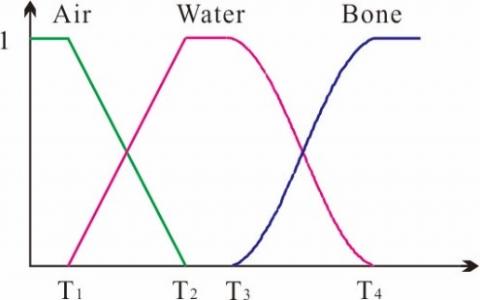
On the CT image (Figure 2), each pixel can be segmented proportionally into three equivalent tissues, namely, the air, water and bone by the proportional division function (Figure 1). The percentages of the three equivalent tissues add up to 1. In this way, the CT image can be completely divided into the three equivalent tissues.
Let $T_{1}, T_{2}, T_{3}$ and $T_{4}$ be $-1,000$ Hounsfield units (HU), OHU, $100 \mathrm{HU},$ and $1,300 \mathrm{HU},$ respectively. Then, our proportional division function takes $T_{1}$ as the upper limit for the air, $T_{4}$ as the lower limit for the bone, and $T_{2} \sim T_{3}$ as the interval for water. For example, a pixel with $\mathrm{CT}$ value smaller than $T_{1}$ is $100 \%$ air, a pixel with CT value greater than $T_{4}$ is $100 \%$ bone, a pixel with CT value between $T_{2}$ and $T_{3}$ is $100 \%$ water, and a pixel with $\mathrm{CT}$ value between $T_{3}$ and $T_{4}$ is a mixture of water and bone.
Here, the pixels with CT values in $\left[T_{3}, T_{4}\right]$ are segmented nonlinearly to determine the percentages of water and bone. The nonlinear segmentation is adopted for the mixture of water and bone rather than linear segmentation, because the latter ignores the difference in X-ray attenuation in water and bone (the X-ray attenuates greater in bone than in water with the same thickness). Through nonlinear segmentation, the CT image can be divided into the equivalent tissues of water, bone and the air, respectively denoted as $W_{w}, W_{b}$ and $W_{a}:$
$W_{w}=\left\{\begin{array}{rlrl}{\frac{\mathrm{z}-\mathrm{T}_{1}}{\mathrm{T}_{2}-\mathrm{T}_{1}}} & &{\mathrm{T}_{1}} & {\leq \mathrm{z}<\mathrm{T}_{2}} \\ {1} && {\mathrm{T}_{2}} & {\leq \mathrm{z}<\mathrm{T}_{3}} \\ {\cos ^{2}\left(\frac{\pi}{2} * \frac{\mathrm{z}-\mathrm{T}_{3}}{\mathrm{T}_{4}-\mathrm{T}_{3}}\right)} && &{\mathrm{T}_{3} \leq \mathrm{z}<\mathrm{T}_{4}}\end{array}\right.$ (1)
$W_{b}=\left\{\begin{array}{cc}{0} & {\mathrm{z}<\mathrm{T}_{3}} \\ {\sin ^{2}\left(\frac{\pi}{2} * \frac{\mathrm{z}-\mathrm{T}_{3}}{\mathrm{T}_{4}-\mathrm{T}_{3}}\right)} & {\mathrm{T}_{3} \leq \mathrm{z}<\mathrm{T}_{4}} \\ {1} & {\mathrm{z} \geq \mathrm{T}_{4}}\end{array}\right.$ (2)
where, Z is the CT value of a pixel.
Figure 1. The proportional division function for equivalent tissue
Figure 2. (A) The original image $f_{0},(\mathrm{B})$ the equivalent tissue of water $W_{w},(\mathrm{C})$ the equivalent tissue of bone $W_{b}$
2.2 Construction of the projection model
If an object is radiated by a monochromatic ray source with the energy $E_{0},$ the monochromatic projection q will have a simple linear relationship with the thickness x penetrated by the X-ray [ 15]:
$\mathrm{q}=\int_{0}^{\mathrm{D}} \mu\left(E_{0}, \mathrm{x}\right) \mathrm{d} \mathrm{x}$ (3)
where, $D$ is the total length of the penetration path of the Xray; $\mu\left(E_{0}, \mathrm{x}\right)$ is the sectional distribution function of the linear attenuation coefficient of the object under $E_{0} .$
For low-energy rays, the attenuation is obvious in water and bone, but weak in the air. In fact, the attenuation of these rays in water and bone is the primary cause of hardening. Hence, this paper neglects the influence of the air on hardening, and only considers that from water and bone. Then, forward projection was preformed based on the three equivalent tissues to set up the projection model for image correction. The specific process is introduced below:
Let $L_{w}$ and $L_{b}$ be the length of the forward projections of the equivalent tissues of water and bone, respectively. During the CT scan, each X-ray penetrates through water and bone, Ieaving a projection $P$ on the detector. In ideal situation, the $\mathrm{X}$ -ray is polychromatic. Then, $P$ must be linearly correlated with $L_{w}$ and $L_{b} .$ In real-world scenarios, the X-ray is polychromatic, and $P$ is actually nonlinearly correlated with $L_{w}$ and $L_{b} .$ The nonlinear terms include the high-order term of bone, the high-order term of water, and their cross term. The high-order term of bone and that of water induce the hardening artefacts of bone and water, respectively.
Theoretically, the polychromatic projection can be described as:
$\mathrm{P}=\mathrm{c}_{1} \mathrm{L}_{\mathrm{w}}+\mathrm{c}_{2} \mathrm{L}_{\mathrm{b}}+\mathrm{c}_{3} \mathrm{L}_{\mathrm{b}}^{2}+\mathrm{c}_{4} \mathrm{L}_{\mathrm{wb}}+\mathrm{c}_{5} \mathrm{L}_{\mathrm{w}}^{2}$ (4)
By formula $(4),$ the $L_{b} \times L_{b}$ and $L_{w} \times L_{b}$ were calculated, and respectively denoted as $\mathrm{L}_{\mathrm{b}}^{2}$ and $\mathrm{L}_{\mathrm{wb}}$.
In this paper, the test data are obtained from a CT scanner. The water hardening artefacts have been corrected [12, 16]. Therefore, only bone hardening artefacts need to be corrected. On this basis, the trinomial fitting model was proposed to fit the polychromatic projection:
$\mathrm{P}=\mathrm{c}_{1} \mathrm{L}_{\mathrm{w}}+\mathrm{c}_{2} \mathrm{L}_{\mathrm{b}}+\mathrm{c}_{3} \mathrm{L}_{\mathrm{b}}^{2}$ (5)
To verify the superiority of the proposed model, another polychromatic projection fitting model was designed for comparison:
$\mathrm{P}=\mathrm{c}_{1} \mathrm{L}_{\mathrm{w}}+\mathrm{c}_{2} \mathrm{L}_{\mathrm{b}}+\mathrm{c}_{3} \mathrm{L}_{\mathrm{b}}^{2}+\mathrm{c}_{4} \mathrm{L}_{\mathrm{wb}}$ (6)
Formula (6) is a quartic polynomial fitting model, including the cross term of water and bone $\mathrm{L}_{\mathrm{wb}}$. The trinomial fitting model and the quartic polynomial fitting model were both applied to hardening correction.
2.3 Coefficient solving
The original image $f_{0}$ was subjected to Radon transform to obtain the projection data $\mathrm{p}_{0} .$ Then, the polychromatic projection $P$ obtained by formula (5) was used to approximate the actual projection p. Due to the lack of raw data, the actual projection was replaced with the projection data p_ acquired by Radon transform. The replacement is reasonable because Radon transform is a parallel linear transform.
Then, the unknown coefficients $c_{1}, c_{2}$ and $c_{3}$ can be determined by the L.S method:
$\mathrm{E}=\min \iint\left(\mathrm{P}-\mathrm{p}_{0}\right)^{2} \mathrm{d} \mathrm{xdy}$ (7)
The coefficients can be derived by:
$\nabla_{c} \mathrm{E}=\nabla_{c} \iint\left(\mathrm{P}-\mathrm{p}_{0}\right)^{2} \mathrm{d} \mathrm{x} \mathrm{d} \mathrm{y}=0$ (8)
The values of $c_{1}, c_{2}$ and $c_{3}$ can be determined by solving the linear equations. Then, the projection of the nonlinear error Perror can be obtained as
$\mathrm{P}_{\text {error }}=\mathrm{c}_{3} \mathrm{L}_{\mathrm{b}}^{2}$ (9)
Next, the Perror was subtracted from the original projection P0 , creating the corrected monochromatic projection $P_{\text {final }}$:
$\mathrm{P}_{\text {final }}=\mathrm{p}_{0}-\mathrm{P}_{\text {error }}$ (10)
Finally, the $P_{\text {final }}$ was reconstructed to obtain the corrected CT image without hardening artefact $\mathrm{f}_{\text {final }}$.
The test objects were scanned by a cone-beam spiral CT scanner produced by Beijing Arrays Medical Imaging Corporation (AMIC), China, at the bulb voltage of 120kVp, the bulb current of 280mA, the medium thickness of 1.25mm, the source-detector distance of 988mm and the source-patient distance of 560mm. The convolution kernel was reconstructed before use.
Both water and polyvinyl chloride (PVC) were adopted for our experiments, because of the similarity in X-ray attenuation between water and soft tissues, and between PVC and human bones. Specifically, two cylindrical buckets were selected, respectively 20cm and 30cm in diameter. Two pure PVC rods (diameter: 30mm) were adopted (SIMONA, Germany).
Before the experiments, the CT scanner has been fully calibrated, including air calibration and water pre-calibration. In the first experiment, the two PVC rods were placed symmetrically around the water-filled bucket (diameter: 20cm), and the experimental model was scanned by the head scan protocol, aiming to simulate the hardening artefacts in human head. In the second experiment, the two PVC rods were placed symmetrically around the water-filled bucket (diameter: 30cm), and the experimental model was scanned by the body scan protocol, aiming to simulate the hardening artefacts in human body. In the third experiment, the head of the subject (a patient) was scanned by the head scan protocol to obtain the clinical data. During the scan, the subject was asked to lie flat on the scanning table.
The experimental model and the patient were scanned by the cone-beam spiral CT scanner, and the obtained scan data were used to evaluate the effectiveness of our model.
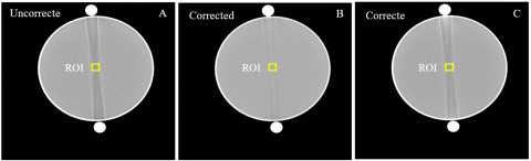
Figure 3 presents the pre- and post-correction results of the first experiment. In the pre-correction image (Figure 3A), there was an obvious stripe artefact between the high attenuators (PVC rods). By contrast, the stripe artefact between the high attenuators basically disappeared in the image corrected by the trinomial fitting model (Figure 3B). This agrees with the result in Kyriakou’s research [12]. Obvious artefact reduction was observed in the image corrected by the quartic polynomial fitting model (Figure 3C).
Figure 3. The pre- and post-correction results of the first experiment
To quantify the accuracy of the two correction models, the first region of interest (ROI1) was identified in the pre- and post-correction images. The mean CT values in ROI1 in the original and corrected images were computed (Table 1).
Table 1. Mean CT values in ROI1 before and after correction
|
Image |
ROI |
Mean CT value |
|
Original image A |
ROI1 |
-22 |
|
Image corrected by trinomial fitting B |
ROI1 |
-4 |
|
Image corrected by quartic polynomial fitting C |
ROI1 |
-12 |
Figure 4 displays the pre- and post-correction results of the second experiment. In the pre-correction image (Figure 4A), there was an obvious stripe artefact between the high attenuators (PVC rods). However, the stripe artefact between the high attenuators was no longer observable in the image corrected by the trinomial fitting model (Figure 4B). This is consistent with the result in Kyriakou’s research [12]. Similarly, the artefact was also greatly reduced in the image corrected by the quartic polynomial fitting model (Figure 4C).
Figure 4. The pre- and post-correction results of the second experiment
To quantify the accuracy of the two correction models, the second region of interest (ROI2) was plotted in the pre- and post-correction images. The mean CT values in ROI2 in the original and corrected images were computed (Table 2).
As shown in Table 2, the mean CT value of ROI2 in the original image was -15HU, which severely deviates from the normal interval of CT values in water (0±4HU). Through trinomial fitting, the mean CT value of ROI2 increased from -15HU to -2HU; through quartic polynomial fitting, the mean CT value of ROI2 increased from -15HU to -9HU. Thus, the mean CT value was increased by both models. The difference is that the mean CT value corrected by trinomial fitting returned to the normal interval (0±4HU), while that corrected by quartic polynomial fitting did not. Therefore, proposed trinomial fitting model is more effective than the other model in hardening correction.
Table 2. Mean CT values in ROI2 before and after correction
|
Image |
ROI |
Mean CT value |
|
Original image A |
ROI2 |
-15 |
|
Image corrected by trinomial fitting B |
ROI2 |
-2 |
|
Image corrected by quartic polynomial fitting C |
ROI2 |
-9 |
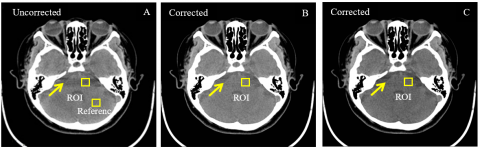
Figure 5. The pre- and post-correction results of the third experiment
In addition, the third region of interest (ROI3) was selected in the pre- and post-correction images. Table 3 records the changes in the mean CT value of ROI3 through the correction.
Table 3. Mean CT values in ROI3 before and after correction
|
Image |
ROI |
Mean CT value |
|
Original image A |
ROI3 |
20 |
|
Image corrected by trinomial fitting B |
ROI3 |
37 |
|
Image corrected by quartic polynomial fitting C |
ROI3 |
25 |
To sum up, both correction methods can remove the hardening artifacts. However, quantification analysis shows that the trinomial fitting model restored the true value of the data. From the perspective of precision medicine, the correction by this model improves the authenticity and reliability of the data. Hence, the proposed trinomial fitting model is an effective way to correct the projection data.
This paper proposes a reverse reconstruction beam hardening correction method, called trinomial fitting model, based on equivalent tissue length. The proposed method does not require information on spectrum and detector. The trinomial fitting model was proved effective in removing hardening artefacts through three experiments. The correction effect is comparable to that of empirical beam hardening correction (EBHC).
Because only water and bone are considered, the equivalent tissues were identified by a simple nonlinear proportional division function, which takes account of the X-ray attenuation difference in water and bone. The division function can be replaced by other division approaches, such as the division method based on regional growth.
The proposed trinomial fitting model for hardening correction uses the data, which had been subjected to water pre-calibration. In real-world scenarios, the clinical CT data are generally processed by water pre-calibration. Therefore, our model can be directly applied to correct the hardening artefacts in clinical data.
This paper suggests correcting beam hardenings based on equivalent tissues, and develops a trinomial fitting model and a quartic polynomial fitting model for projection correction. The two models were tested by the data of experimental model and clinical data. The test results show that the proposed trinomial fitting model for projection correction, which is based on equivalent tissue length, is an effective way to remove the hardening artefacts of X-rays, and a universally applicable approach for various test materials. The proposed model can be adopted for hardening correction of any polychromatic CT system, without requiring any prior knowledge of scanning.
During image correction, the proposed trinomial fitting model has many advantages in calculation, namely, the limited number of parameters, and the simple, fast process. Moreover, our model corrects the artefacts through fitting based on equivalent tissue length, which is correct and clear in physical meanings. There are various potential application fields of our model, such as the precise quantitative analysis of clinical CT, radiotherapy planning and interventional CT research. The research results lay a solid basis for subsequent machine learning based on artificial intelligence.
[1] Bracewell, R.N., Riddle, A. (1967). Inversion of fan-beam scans in radio astronomy. The Astrophysical Journal, 150: 427-434.
[2] Как, A.C., Slaney, M. (1988). Principles of computerized tomographic imaging. The Institute of Electrical and Electronics Engineers, Inc.
[3] Gao, H., Zhang, L., Chen, Z., Xing, Y., Li, S. (2006). Beam hardening correction for middle-energy industrial computerized tomography. IEEE Transactions on Nuclear Science, 53(5): 2796-2807. https://doi.org/10.1109/TNS.2006.879825
[4] Marshall Jr, W.H., Alvarez, R.E., Macovski, A. (1981). Initial results with prereconstruction dual-energy computed tomography (PREDECT). Radiology, 140(2): 421-430. https://doi.org/10.1148/radiology.140.2.7255718
[5] Maaß, C., Meyer, E., Kachelrieß, M. (2011). Exact dual energy material decomposition from inconsistent rays (MDIR). Medical Physics, 38(2): 691-700. https://doi.org/10.1118/1.3533686
[6] Nalcioglu, O., Lou, R.Y. (1979). Post-reconstruction method for beam hardening in computerised tomography. Physics in Medicine & Biology, 24(2): 330-340. https://doi.org/10.1088/0031-9155/24/2/009
[7] Joseph, P.M., Ruth, C. (1997). A method for simultaneous correction of spectrum hardening artifacts in CT images containing both bone and iodine. Medical Physics, 24(10): 1629-1634. https://doi.org/10.1118/1.597970
[8] Van Gompel, G., Van Slambrouck, K., Defrise, M., Batenburg, K.J., De Mey, J., Sijbers, J., Nuyts, J. (2011). Iterative correction of beam hardening artifacts in CT. Medical Physics, 38(S1): S36-S49. https://doi.org/10.1118/1.3577758
[9] Zhao, Y., Li, M. (2015). Iterative beam hardening correction for multi-material objects. PloS One, 10(12): e0144607. https://doi.org/10.1371/journal.pone.0144607
[10] Herman, G.T. (1979). Correction for beam hardening in computed tomography. Physics in Medicine & Biology, 24(1): 81-106. https://doi.org/10.1088/0031-9155/24/1/008
[11] Kachelrieß, M., Sourbelle, K., Kalender, W.A. (2006). Empirical cupping correction: A first‐order raw data precorrection for cone‐beam computed tomography. Medical Physics, 33(5): 1269-1274. https://doi.org/10.1118/1.2188076
[12] Kyriakou, Y., Meyer, E., Prell, D., Kachelrieß, M. (2010). Empirical beam hardening correction (EBHC) for CT. Medical Physics, 37(10): 5179-5187. https://doi.org/10.1118/1.3477088
[13] Chen, C.Y., Chuang, K.S., Wu, J., Lin, H.R., Li, M.J. (2001). Beam hardening correction for computed tomography images using a postreconstruction method and equivalent tisssue concept. Journal of Digital Imaging, 14(2): 54-61. https://doi.org/10.1007/s10278-001-0003-2
[14] Shanghai Lianying Medical Technology Co, Ltd. A correction method of bone hardening artifacts in CT image reconstruction: in Chinese, CN 103186883 A[p]. 2013.07.03
[15] Kijewski, P.K., Bjärngard, B.E. (1978). Correction for beam hardening in computed tomography. Medical Physics, 5(3): 209-214. https://doi.org/10.1118/1.594429
[16] Schüller, S., Sawall, S., Stannigel, K., Hülsbusch, M., Ulrici, J., Hell, E., Kachelrieß, M. (2015). Segmentation‐free empirical beam hardening correction for CT. Medical Physics, 42(2): 794-803. https://doi.org/10.1118/1.4903281