Behnam Asghari Beirami* | Mehdi Mokhtarzade
© 2019 IIETA. This article is published by IIETA and is licensed under the CC BY 4.0 license (http://creativecommons.org/licenses/by/4.0/).
OPEN ACCESS
Random patches network (RPNet) is an emerging deep learning method that can effectively extract the deep features from hyperspectral images. However, this network only relies on spectral bands in feature extraction, failing to make use of the information-rich spatial features. This paper puts forward another variant of the RPNet, named G-RPNet. The proposed network extracts the deep hierarchical Gabor features, with Gabor spatial features as inputs. The extracted deep hierarchical features were stacked to those extracted by the RPNet, and the final feature vectors were classified by the support vector machine (SVM). The integrated feature vectors inherit the merits of the deep hierarchical features of both RPNet and G-RPNet, laying a solid basis for the classification of hyperspectral images. Experiments were conducted on two real hyperspectral images (Indian Pines and Pavia University) from agricultural and urban areas. The results prove the superiority of the proposed method in the classification of hyperspectral images over some recent shallow and deep spatial-spectral classification techniques.
hyperspectral classification, random patches network, Gabor filter, support vector machine
Due to wealth spectral characteristics, hyperspectral images (HSI) are used in various fields such as agriculture, mineralogy, military, medicine, and urban planning. Although many advanced methods are proposed in the literature for feature extraction from HSI, how to exploit discriminative spectral-spatial features from this rich source of data is still a critical challenge.
Based on the literature, different feature extraction methods such as principal component analysis (PCA), minimum noise fraction (MNF), independent component analysis (ICA) and wavelet decomposition and linear discriminant analysis (LDA) are proposed for extracting the spectral features of hyperspectral images. Due to the spectral confusion of similar pixels and the problem of mixed pixels, the classification of HSI with only spectral features may lead to noisy classified maps. To address this issue, a set of techniques are developed which use spatial features such as shape and texture of the image to improve the performance of pixel-based classifiers.
Gray level co-occurrence matrix (GLCM) [1], Gabor filter banks [1], local binary pattern (LBP) [2], morphological profiles [3], attribute profiles [4], local surface fitting features (LSFFs), and image moments [5] are among the most important methods for generating the spatial features. As a core idea, these spatial features are generated before classification in the stage of spatial feature generation and then stacked to spectral features and classified via a robust classifier such as support vector machines (SVM) because of its ability to handle the high dimensional feature vectors. In this direction, the multiple spatial features (morphological profiles, Gabor features and GLCM features) are combined with spectral features and final spatial-spectral features vectors are classified via SVM [6].
Recently, deep learning is an active topic in the HSI classification concept because of its ability for extracting the deep features which are more robust and discriminative in comparison to shallow features. Until now, many deep learning models are proposed for the classification of HSI. As the first attempts in literature, Chen et al. [7] proposed the stacked Autoencoder (SAE) for extracting the deep spatial-spectral features of HSI. Improved Autoencoder model named stacked sparse Autoencoder (SSAE) is proposed by Tao et al. [8]. The Deep belief network (DBN) is introduced by Chen et al. [9] based on a singular restricted Boltzmann machine to learn the shallow and deep features of HSI. A convolutional neural network (CNN) is adopted for the classification of HIS [10]. In this model, CNN is trained via spatial patches around each labeled pixel, and then the trained model predicts the label of each test pixel based on surrounding pixels. PCANet is proposed by Chan et al. [11] in which PCA transform is used to learn the convolutional kernels and then extracted deep features are classified via SVM.
As the recent trend, spatial features (i.e. attribute profiles and Gabor features) are used in combination with deep models [4, 12]. This is motivated by the ability of deep models to extract more abstract and robust features from shallow spatial features. Despite the appropriate performance of deep models in the classification of HSI, there are still some issues that should be addressed: Computational burden is the first issue that decreases the applicability of deep models. As another issue, in many deep learning models, the deepest level of features (features from the last network layer) in the network is used in the Softmax layer for the analysis of HSI. For example, Aptoula et al., based on their flowchart, only the deep features of the third convolution layer are used in the fully connected layer for classification of HIS and the other deep features of first convolution layer and second convolution layer are discarded [4].
These two major issues are addressed in some new studies. Zhao et al. [13] proposed a novel framework named multiple convolutional layers fusion (MCLF) which can exploit different levels of deep features in the classification of HSI. Rotation based deep forest (RBDF) is proposed by Cao et al. [14] in which the output probability of each layer is used as the supplement feature of the next layer, and rotation forest is used to increase the discriminative power of features. As a recent study, the random patches network (RPNet) is proposed by Xu et al. [15] that simulates a deep model with the principal component analysis and convolutional kernels that are directly extracted from image random patches without any training stage.
Although the original RPNet has an excellent ability for extracting the deep features from different layers of deep network with a low-computational burden, it only uses the original spectral bands as the input features. In other words, the original RPNet neglects the spatial features as another rich source of data. Motivated from the ability of Gabor filter banks to extract the image objects from different scales and orientations, in this study we introduce the new variant of RPNet, named G-RPNet, based on Gabor features. In G-RPNet, Gabor spatial features which are produced from different scale and orientation are used as the input of RPNet and deep Gabor features are extracted from different layers of the network. To put in a nutshell, the main contributions of this paper are as follows:
• This paper, motivated by the ability of Gabor filter banks in spatial feature extraction from different directions and scales, G-RPNet is proposed which uses the Gabor features as inputs to extract the hierarchical deep Gabor features.
• As an innovative point, a method named SGDFF (Spectral-Gabor Deep Features Fusion) is proposed in this paper in which extracted deep features of G-RPNet are stacked with deep features of the original RPNet. SGDFF takes advantage of both shallow/ hierarchical deep Gabor-spectral features.
In section 2, we summarize the concepts of Gabor filters, SVM, and introduce the G-RPNet and the method of combining the deep spatial-spectral features. Section 3 introduces the two hyperspectral images which are used in experiments. Section 4 reports the results of classification followed by discussions. Moreover, last section 5 concludes the study.
2.1 Gabor features
Gabor features as spatial features are used to extract image objects in different directions and scales. The core of the Gabor feature extraction method is the 2D Gabor filter function that is shown in the spatial domain as below [16, 17]:
$\phi(x, y)=\frac{f^{2}}{\pi \gamma \mu} e^{-\left(\frac{f^{2}}{\gamma^{2}} x^{\prime 2}+\frac{f^{2}}{\gamma^{2}} y^{\prime 2}\right)+j 2 \pi f x^{\prime}}$
$\begin{aligned} x^{\prime} &=x \cos (\theta)+y \sin (\theta) \\ y^{\prime} &=-x \sin (\theta)+y \cos (\theta) \end{aligned}$ (1)
in which, f is the filter tuning frequency and γ, μ control the bandwidth which corresponds to two perpendicular axes of Gaussian. θ is the rotation angle of both Gaussian and plane wave. Fourier transformed version function (1) has the following Eq. (2) in the frequency domain [16, 17]:
$\begin{aligned} \phi(u, v) &=e^{-\pi^{2}\left(\frac{u^{\prime}-f}{\alpha^{2}}+\frac{v^{\prime}}{\beta^{2}}\right)} \\ u^{\prime} &=u \cos (\theta)+v \sin (\theta) \\ v^{\prime} &=-u \sin (\theta)+v \cos (\theta) \end{aligned}$ (2)
which is the single Gaussian band-pass filter. Gabor features are constructed from responses of Gabor filters (1) or (2), commonly, in different directions and scales. Output values of Gabor filter are complex, and usually, its magnitude is used. Due to the high dimensionality of HSI in this study, Gabor features are generated from the first three principal components of HSI (which contain above 95% of variance).
MATLAB image processing toolbox is carried out for generating the Gabor features in the four directions [0, 45, 90, 135] and 24 scales (in MATLAB, wavelength values in the range [2:25]). Based on this setting, a total of 288 Gabor features are generated from the first three principal component analysis features (PCs) for each data set and are used in experiments.
2.2 G-RPNet
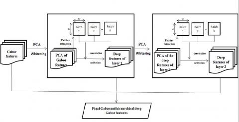
In RPNet, there is no training stage, despite the traditional deep learning. In this model, random patches that contain the useful geometrical and textural information are selected from the image and are used as the convolution kernels. G-RPNet, as a variant of original RPNet, uses the Gabor features from different scale and orientation as inputs to extract the hierarchical deep Gabor features. G-RPNet same as RPNet has two major layers, including principal component analysis (PCA) and data whitening, and convolution with random patch selection and rectified linear units (ReLU). More details of these layers are as follows [15]:
To reduce the computation burden of the model, PCA is used for the features extraction of each layer of RPNet. In order to create the features with similar variances and to decrease the correlations of the features, the whitening operation is applied to p extracted features of the PCA layer.
In the next layer, we randomly selected the k pixels from whitened data, and the k patches around them with size w×w×p are used as convolutional kernels. As so, we can get the k features maps with convolving the p whitened images with k convolutional kernels as follows:
$I_{i}=\sum_{j=1}^{p} X_{\text {whitened }}^{j} * P_{i}^{j}, i=1, \ldots, k$ (3)
where, * denotes the convolution operation, Ii is the ith feature map, $X_{\text {whitened }}^{j}$ is the jth band of whitened data and $P_{i}^{j}$ is the jth dimension of the ith random patch. Convolutional kernels are slide in all over the image with a stride of 1, and mirror extension is used for pixels in the edge of the image. For improving the sparsity of features, G-RPNet, the same as RPNet, uses the rectified linear unit (ReLu) as the activation function.
G-RPNet with two deep layers is shown in Figure 1. Based on this figure, original Gabor features (Gi) and deep Gabor features from different deep layers (hierarchical deep Gabor features, DGi) are stacked and considered as final features vectors of G-RPNet. The final feature vector in each pixel (i,j) is shown below:
$G-R P N e t_{(i, j)}=\left[G_{1} ; \ldots, G_{R} ; D G_{1} ; D G_{2} ; \ldots ; D G_{l}\right]$ (4)
R is the number of original Gabor features and l is the number of hierarchical deep Gabor features.
Figure 1. Flowchart of G-RPNet
2.3 Support vector machines
Support vector machines (SVM), as the non-parametric supervised classifier, is widely used for classification of high dimensional data, such as HSI, because of its excellent performance and its ability to handle the high dimensional data. SVM classifies the data based on maximizing the geometrical margin and minimizing the empirical error. In the context of HSI classification, commonly, kernel trick is used to map the data to the higher dimensional space in which data are linearly separable. Given p training sample [(x1,y1),(x2,y2),…,(xp,yp)] in which xp is the N-dimensional vector correspond to N features and yp is the class labels {-1,+1}. To classify the data with SVM, the following function should be maximized with respect to $\alpha_{i}$ (Lagrange multipliers) [18]:
$L=\sum_{i} \alpha_{i}+\frac{1}{2} \sum_{i, j} \alpha_{i} \alpha_{j} y_{i} y_{j}\left(x_{i} x_{j}\right)$ (5)
Given non-linear mapping ϕ(x) [19] Eq. 5 can be represented by:
$L=\sum_{i} \alpha_{i}+\frac{1}{2} \sum_{i, j} \alpha_{i} \alpha_{j} y_{i} y_{j}\left(\phi\left(x_{i}\right) . \phi\left(x_{j}\right)\right)$ (6)
A kernel function is defined as:
$K=\phi\left(x_{i}\right) . \phi\left(x_{j}\right)$ (7)
By substituting (7) in (6) and solving the problem, SVM decision function for test sample x is shown as:
$f(x)=\operatorname{sign}\left(\sum_{i=1}^{p} y_{i} \alpha_{i} K\left(x_{i}, x\right)+b\right)$ (8)
in which, b is computed from $\alpha_{i}$. In this study, cubic polynomial kernel with the following formula is used to classify of spatial-spectral features [5]:
$K\left(x_{1}, x_{2}\right)=\left(\frac{1}{\text { number of features }} x_{1} x_{2}^{T}\right)^{3}$ (9)
$x_{1}, x_{2}$ are the two arbitrary feature vector, and T vector transpose. Also, each feature vector is mapped to [-255,255]. It is worth to note that, SVM is inherently a two-class classifier that is extended to the multiclass problem by two techniques named "one against one" and "one against all".
2.4 Stacking the G-RPNet and RPNet features
As mentioned before, the original RPNet can only extract the hierarchical deep features based on spectral features and ignores the spatial features as the inputs. To address this issue in this study, G-RPNet is proposed that uses the Gabor features as the inputs of RPNet to extract the hierarchical deep Gabor features. Due to complement characteristics of Gabor and spectral features, the SGDFF method is proposed in this study. Final feature vectors of SGDFF consist of stacking the extracted features of RPNet and G-RPNet. In other words, the feature vector of RPNet and SGDFF for every pixel (i, j) are shown below:
$R P N e t_{(i, j)}=\left[b_{1} ; b_{2} ; \ldots ; b_{N} ; D b_{1} ; D b_{2} ; \ldots ; D b_{S}\right]$ (10)
$S G D F F_{(i, j)}=\left[R P N e t_{(i, j)} ; G-R P N e t_{(i, j)}\right]$ (11)
In (10) bi indicates the original spectral bands, N is the numbers of original bands, $D b_{i}$ is the hierarchical deep features which are extracted via RPNet, S is the numbers of RPNet deep features. Then, final vectors of SGDFF are classified via SVM because of its ability to handle the high dimensional data.
Two real hyperspectral images, Indian Pines and Pavia University, are used in this study. Their details are as follows.
3.1Indian pines
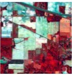
This hyperspectral image is collected by the AVIRIS sensor in 1992 from Indianapolis in the USA. After removing the noisy and water absorption bands, the remaining 200 spectral bands are used in experiments. The size of the image is 145×145 pixels, and the spatial resolution is 20 meters. This scene contains the 16 agricultural classes such as soybean, corn, etc. a false-color image of this scene is shown in Figure 2.
Figure 2. Indian pines hyperspectral image
3.2 Pavia University
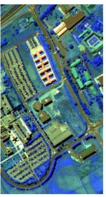
This hyperspectral image is collected by ROSIS 3 sensor from Pavia University in northern Italy. After removing the noisy and water absorption bands, the remaining 103 spectral bands are used in experiments. The size of the image is 610×340 pixels, and the spatial resolution is 1.3 meters. This urban scene contains the nine class of information such as asphalt, bitumen, etc. a false-color of this scene is shown in Figure 3.
Figure 3. Pavia University hyperspectral image
Experiments of this study are conducted on two real hyperspectral images Indian pines and Pavia University. For both data sets, two sizes of training samples, 5%, and 10%, of the ground truth are randomly selected as training samples, and remaining samples of ground truth are considered as test samples. In all experiments mean of the classification overall accuracies of ten times running of the method with different sets of training and test samples are reported. MATLAB 2019a is used for the implementation of all experiments. SVM is implemented based on LibSVM [20].
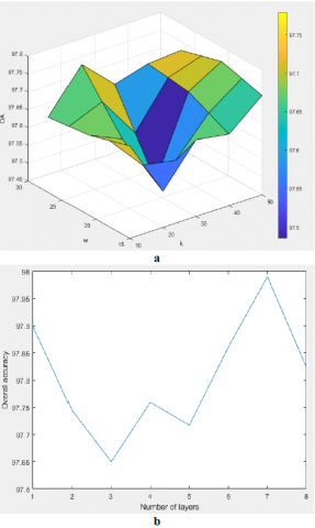
4.1 Parameters analysis
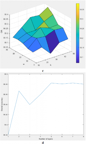
Same as RPNet, G-RPNet has three important parameters including, the size of the patches (w), number of the random patches (k), and depth or the number of the network layers. To investigate the impacts of these parameters, in the first experiment of this section the depth of the G-RPNet for both data is set as 1 and the performance of G-RPNet for both data are studied with different values of w and k. Extracted features of each case are classified in the situation of 10% of training samples via SVM, and results for both data set are shown in Figure 4. a, and 4. c. The analyses of results are summarized as follows:
Figure 4. Parameters analysis of G-RPNet- a, b) Indian Pines- c, d) Pavia University
In the second experiment by considering the optimum values of w and k for each data set, we investigate the impact of depth or the number of layers. Classification results when a different number of layers are considered for both data sets are shown in Figure 4. b and 4. d. The plot of Indian Pines has some fluctuation, and the best result is obtained when a number of layers is 7 but for Pavia University best result is obtained in 5 and after that adding the more layers has no impact on results.
4.2 Results and discussions
To evaluate the efficiency of the proposed method for classification of hyperspectral images, in this section we compare the classification result of the proposed method (G-RPNet and SGDFF) with other spatial-spectral classification methods which their more descriptions are as follows:
Final overall classification accuracies of proposed methods and other competitor methods are reported in Table 1. The analyses of results are summarized as follows:
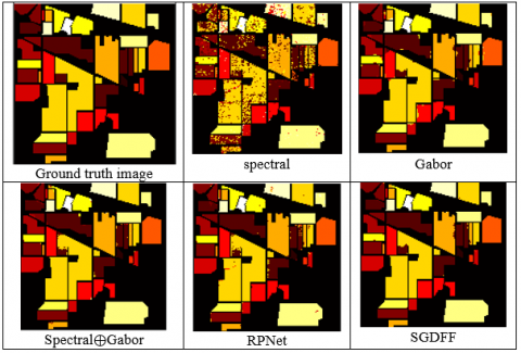
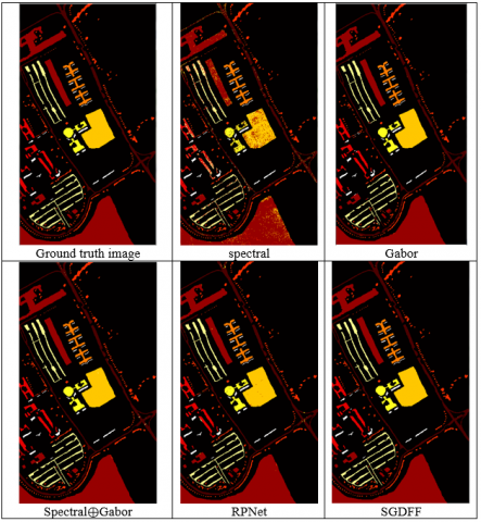
This experiment proved that SGDFF that takes advantage of both deep spectral and spatial features is an excellent method for the classification of HSIs both from agricultural and urban areas. For the sake of visual comparison, classified images of proposed SFDFF and other methods (which are implemented by authors) for the situation of 10% training samples are shown in Figure 5 and Figure 6 for both data sets. Based on these figures, we can say that SFDFF produced the smoothest classified maps with the lowest levels of salt and paper noise.
All experiments are implemented with a desktop computer with specifications of Intel(R) Core(TM) i5-6400 CPU and 8.00 GB RAM. Processing times of features generation for Pavia university in SGDFF is about 50 seconds which is five times higher than the original RPNet with 10 seconds. Although proposed SGDFF is not superior in the computational times in comparison to some methods (i.e. Spectral, Gabor, Spectral $\oplus$ Gabor, SSTF, RPNet), it is still faster than most of the deep learning methods (i.e. RBDF with 693 seconds).
Table 1. Comparison with other methods
|
Method |
Training samples size |
||||
|
10% |
5% |
||||
|
Indian Pines |
Pavia University |
Indian Pines |
Pavia University |
||
|
Spectral |
79.30 |
89.76 |
73.38 |
89.95 |
|
|
Gabor |
97.91 |
98.64 |
93.93 |
97.79 |
|
|
Spectral $\oplus$ Gabor |
98.55 |
99.71 |
96.59 |
99.49 |
|
|
SSTF (2015) [6] |
96.48 |
99.37 |
92.78 |
98.95 |
|
|
Moment (2016) [5] |
NA* |
99.82 |
NA* |
99.60 |
|
|
FCLFN (2019) [13] |
98.56 |
NA* |
≈96 |
NA* |
|
|
RBDF (2019) [14] |
NA* |
99.52 |
NA* |
99.42 |
|
|
RPNet (2018) [15] |
97.76 |
99.26 |
95.46 |
98.88 |
|
|
Proposed |
G-RPNet |
97.98 |
99.48 |
94.97 |
98.52 |
|
SGDFF |
99.12 |
99.93 |
97.34 |
99.84 |
|
|
NA*: In this situation, results of classification are not reported in the source paper. |
|||||
Figure 5. Indian pines classified image with different methods
Figure 6. Pavia university classified image with different methods
In this paper, a new variant of RPNet named G-RPNet is proposed that uses Gabor spatial features as the inputs of the network. G-RPNet is used to extract the hierarchical deep spatial features from different orientations and scales. Due to the complementing nature of Gabor and spectral features, extracted features of G-RPNet and original RPNet are stacked and resultant feature vectors are classified via SVM classifier. The final results demonstrate that the proposed method of this study outperforms the other recent methods and has great ability in the classification of hyperspectral images.
In this paper, different Gabor-spectral features are stacked and then classified by SVM, but based on literature; it seems that it is more efficient to combine the different deep features in composite kernel SVM. Therefore, this concept is suggested for future studies.
[1] Imani, M., Ghassemian, H. (2016). GLCM, Gabor, and morphology profiles fusion for hyperspectral image classification. In 2016 24th Iranian Conference on Electrical Engineering (ICEE) IEEE. Shiraz, Iran, pp. 460-465. http://dx.doi.org/10.1109/IranianCEE.2016.7585566
[2] Gao, F., Wang, Q., Dong, J., Xu, Q. (2018). Spectral and spatial classification of hyperspectral images based on random multi-graphs. Remote Sensing, 10(8): 1271. http://dx.doi.org/10.3390/rs10081271
[3] Benediktsson, J.A., Palmason, J.A., Sveinsson, J.R. (2005). Classification of hyperspectral data from urban areas based on extended morphological profiles. IEEE Transactions on Geoscience and Remote Sensing, 43(3): 480-491. http://dx.doi.org/10.1109/TGRS.2004.842478
[4] Aptoula, E., Ozdemir, M.C., Yanikoglu, B. (2016). Deep learning with attribute profiles for hyperspectral image classification. IEEE Geoscience and Remote Sensing Letters, 13(12): 1970-1974. http://dx.doi.org/10.1109/LGRS.2016.2619354
[5] Mirzapour, F., Ghassemian, H. (2016). Moment-based feature extraction from high spatial resolution hyperspectral images. International Journal of Remote Sensing, 37(6): 1349-1361. http://dx.doi.org/10.1080/2150704X.2016.1151568
[6] Mirzapour, F., Ghassemian, H. (2015). Improving hyperspectral image classification by combining spectral, texture, and shape features. International Journal of Remote Sensing, 36(4): 1070-1096.
[7] Chen, Y., Lin, Z., Zhao, X., Wang, G., Gu, Y. (2014). Deep learning-based classification of hyperspectral data. IEEE Journal of Selected Topics in Applied Earth Observations and Remote Sensing, 7(6): 2094-2107. http://dx.doi.org/10.1109/JSTARS.2014.2329330
[8] Tao, C., Pan, H., Li, Y., Zou, Z. (2015). Unsupervised spectral–spatial feature learning with stacked sparse autoencoder for hyperspectral imagery classification. IEEE Geoscience and Remote Sensing Letters, 12(12): 2438-2442. http://dx.doi.org/10.1109/LGRS.2015.2482520
[9] Chen, Y., Zhao, X., Jia, X. (2015). Spectral–spatial classification of hyperspectral data based on deep belief network. IEEE Journal of Selected Topics in Applied Earth Observations and Remote Sensing, 8(6): 2381-2392. https://doi.org/ 10.1109/JSTARS.2015.2388577
[10] Chen, Y., Jiang, H., Li, C., Jia, X., Ghamisi, P. (2016). Deep feature extraction and classification of hyperspectral images based on convolutional neural networks. IEEE Transactions on Geoscience and Remote Sensing, 54(10): 6232-6251. http://dx.doi.org/10.1109/TGRS.2016.2584107
[11] Chan, T.H., Jia, K., Gao, S., Lu, J., Zeng, Z., Ma, Y. (2015). PCANet: A simple deep learning baseline for image classification? IEEE Transactions on Image Processing, 24(12): 5017-5032. http://dx.doi.org/10.1109/TIP.2015.2475625
[12] Kang, X., Li, C., Li, S., Lin, H. (2017). Classification of hyperspectral images by Gabor filtering based deep network. IEEE Journal of Selected Topics in Applied Earth Observations and Remote Sensing, 11(4): 1166-1178. http://dx.doi.org/10.1109/JSTARS.2017.2767185
[13] Zhao, G., Liu, G., Fang, L., Tu, B., Ghamisi, P. (2019). Multiple convolutional layers fusion framework for hyperspectral image classification. Neurocomputing, 339: 149-160. http://dx.doi.org/10.1016/j.neucom.2019.02.019
[14] Cao, X., Wen, L., Ge, Y., Zhao, J., Jiao, L. (2019). Rotation-based deep forest for hyperspectral imagery classification. IEEE Geoscience and Remote Sensing Letters, 16(7): 1-4. http://dx.doi.org/10.1109/LGRS.2019.2892117
[15] Xu, Y., Du, B., Zhang, F., Zhang L. (2018). Hyperspectral image classification via a random patches network. ISPRS Journal of Photogrammetry and Remote Sensing, 142: 344-357. http://dx.doi.org/10.1016/j.isprsjprs.2018.05.014
[16] Ilonen, J., Kamarainen, J.K., Paalanen, P., Hamouz, M., Kittler, J., Kalviainen, H. (2008). Image feature localization by multiple hypothesis testing of Gabor features. IEEE Transactions on Image Processing, 17(3): 311-325. http://dx.doi.org/10.1109/TIP.2007.916052
[17] Jain, M., Sinha A. (2015). Classification of satellite images through Gabor filter using SVM. International Journal of Computer Applications, 116(7): 18-21. http://dx.doi.org/10.5120/20348-2534
[18] Camps-Valls, G., Gomez-Chova, L., Muñoz-Marí, J., Vila-Francés, J., Calpe-Maravilla, J. (2006). Composite kernels for hyperspectral image classification. IEEE Geoscience and Remote Sensing Letters, 3(1): 93-97. http://dx.doi.org/10.1109/LGRS.2005.857031
[19] Cover, T.M. (1965). Geometrical and statistical properties of systems of linear inequalities with applications in pattern recognition. IEEE Transactions on Electronic Computers, EC-14(3): 326-334. http://dx.doi.org/10.1109/PGEC.1965.264137
[20] Chang, C.C., Lin, C.J. (2011). LIBSVM: A library for support vector machines. ACM Transactions on Intelligent Systems and Technology (TIST), 2(3): 27. http://dx.doi.org/10.1145/1961189.1961199