Siva Koteswara Rao Chinnam | Venkatramaphanikumar Sistla* | Venkata Krishna Kishore Kolli
© 2019 IIETA. This article is published by IIETA and is licensed under the CC BY 4.0 license (http://creativecommons.org/licenses/by/4.0/).
OPEN ACCESS
In this study, we propose an efficient method to identify unwanted growth in brain using SVM-PUK on convoluted textural features with reduced Gabor wavelet features. After pre-processing, GLCM features of image are extracted and further, convoluted with reduced Gabor features using PCA of the image. Then, the convoluted GLCM features and reduced Gabor features classified with the SVM using PUK kernel. The proposed method performance is evaluated on BRATS’18 database and achieved an accuracy of 91.31 % in recognizing the effected tissues, and shown better performance over ED, DTW, FFNN and PNN.
brain tumor, statistical features, principle component analysis, Gabor, support vector machine, PUK kernel
In today’s digital scenario, to provide better health care, clinical experts utilizing the e-healthcare systems in diagnosing diseases and in treatment planning. Magnetic resonance Images of Brain provides better 3D vision of structure and gives clarity on infected tissues of human brain neural architecture. Due to appearance, strokes in MRI, position, shape, size, fuzzy boundaries and different intensities it is very challenging to perform automatic segmentation of MRI data. An abnormal growth of brain cells [1], will affect the normal functionality of the brain and destroy the healthy cells. As per WHO, abnormal growth of cell in and around brain is classified as benign (Non-Cancerous), i.e., Low Grade I and II (Uniformity –Very Slow Growth rate - will not affect other parts of body) or malignant (Cancerous), i.e., High Grade III and IV (Non-Uniform – Rapid Growth rate - will affect other parts of body) [2]. Malignant growth is further classified into Primary (originate inside brain) and Secondary (originate another part of the body and propagates towards the brain) based on growth location. Complex structure of the brain is very challenging to diagnose the growth area. In diagnosing abnormal growths, treatment planning and treatment results and evaluation, segmentation plays a crucial role. In segmentation process, based on color, texture, contrast of image and boundaries, divide the image into parts.
Automatic and Semi-Automatic tumor segmentation methods were developed, as manual segmentation involves human errors and are also laborious [3], focusing on gliomas in MRI. Based on appearance, strokes in MRI, position, shape, size, fuzzy boundaries and different intensities it is very challenging to segment MRI data [4]. Enhanced imaging techniques helps in the occurrence, track of growth of tumor-affected regions to provide suitable diagnosis. Early detection of brain tumor is helpful in proper treatment like radiation, surgery or chemotherapy. In the process of diagnosing the tumor, physicians can verify different modalities and identify whether tumor is present or not. If so, to find tumor location and volume of the tumor is laborious task and it needs much attention. Due to time limitations and growth of tumor costs life, it leads to demand for the computer vision in this context that leads to semi-automatic and automatic segmentation. For better control in segmentation process to assure accuracy, radiologists will prefer for semi-automatic segmentation methods over automatic segmentation methods as they need only user initialization and repeated user interaction.
In this paper, Section II describes a detailed literature work. Section III describes about the proposed framework incorporated with machine learning strategies to examine, segment and classify the tumors. Section IV describes the investigational observations. Finally, conclusion is given in Section V.
In the literature, for brain and tissue segmentation various methods were presented [5] and abnormality detection methods in and around brain [6] were proposed. Chi-Hoon Lee et al. [7] proposed Support Vector Random Field (SVRF) Model, that shows better performance in segmentation of tumour over SVM, CRF, DRF, ML, MRF, L R Nilesh Bhaskar rao Bahadure et al. [8] have applied Berkeley Wavelet Transformation (BWT) to segment brain tumours. Then, extracted features from each segmented tissue are classified using SVM and yielded 97 % in terms of accuracy. Arun Garg et al., [9] extracted the features using PCA, applied K-mean for image segmentation then applied SVM for image Classification achieved 96 % accuracy. P Kumar et al., [10] used PCA and RBF Kernel based SVM for segmentation and classification of MR Images that yields classification accuracy of 94 %. Stefan Bauer et al. [11] Fully Automatic Segmentation method uses SVM classification in combination with HCRFR shows a good performance. Marco Alfonse et al., [12] proposed method classifying and then performing segmentation got an accuracy of 98.9 %. Roy et al. [13] have proposed a method helps in detection of MS lesions and segmentation in adaptive background and binarization using global threshold. Ahmmed et al. [14] method enhanced the brain MRI image and then classified using temporal K-means integrated with improved fuzzy C-means. Using SVM and Neural network classifier growth stage was classified and achieved an accuracy of 97.37 % with BER of 0.0294. Amin et al. [15] proposed an automatic method with less processing time, that identifies malignant tissues in MRI Brain and got an average 97.1 %, 98.0 %, 91.9 % and 98.0 % of accuracy, area under curve, sensitivity and specificity respectively. A R Kavitha et al. [16] finds growth using improved region growing and using FFNN and RBF neural network with an accuracy of 80.0 %. T Ramakrishnan et al. [17], classified and segmented the tumor region in CT images with an accuracy 99.05 %. Roy et al. [18] computerized method applies binarization to pre-processing, features extraction and identification of brain abnormality and determines threshold value followed by a non-gamut enhancement, using binarization with help of statistical features like Mean, Variance, Std. dev., and Entropy.
S. Valverde et al. [19] fully automated method in T1-W / FLAIR tissue segmentation deals with images that has WM lesions and performed on the MRBrainS13 challenge database and outperformed over unsupervised pipelines such as FAST and SPM12. A. Vishnu varthanan et al. [20] proposed a totally a robotized approach to find viable tumour isolation and tissue division utilizing the procedures BFO and MFCM calculations into a solitary structure to perform MR cerebrum picture division and affectability and the specificity are 0.9048 and 0.9825, separately. Aye Min et al. [21] fusion method enhanced the 72 Flair images and segments using adaptive k-means clustering, morphological operation on multimodal images of brain tumour leads to TPR of 85.41 %, TNR of 98.90 %, PVP of 78.30 % and with accuracy 98.23 %. Kaya et al. [22] have done comparative study over PCA, Probabilistic PCA, and other variant dimensionality reduction methods prior to K-Means and Fuzzy C-Means on human brain images of size of 512×512, 256 × 256, 128 × 128 and 64 × 64. Their proposed method outperformed among all in terms of the reconstruction, Euclidean distance errors. UmitIlhan et al. [23] proposed a method with morphological operations, followed by pixel subtraction, then threshold-based segmentation and finally various image filtering techniques to obtain clear images of the skull, brain and recognizing tumors with an accuracy of 94.28 % on benchmark images. The Cancer Imaging Archive (TCIA) shows 96.0 % success rate, which shows a better performance in comparison with other methods. Ashwini Sankhe et al. [24] compared SVM and PNN Classifiers using Confusion Matrix and found PNN is outperformed over SVM. Deven Ketkar., [25] compared SVM and PNN Classifiers on datasets and found SVM outperformed over PNN.
The proposed novel approach helps to answer the shortcomings found at literature. Further, performance of the proposed method is evaluated with various wavelets and SVM kernels on BRATS-2018. In this approach the following steps are carried in the classification of brain tumor.
Step 1: Data acquisition
Step 2: Preprocessing of Brain Images
Step 3: Segmentation of Tumor
Step 4: Extraction GLCM and Statistical Features
Step 5: Tumor Classification with SVM.
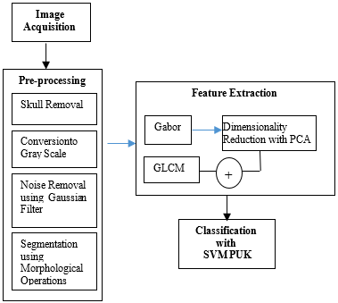
Figure 1. Architecture of the proposed framework
3.1 Pre-processing
Pre-processing step is used by clinical experts on imaging modalities for improving visual appearance of MR images, identification of best features [26]. For the enhancement of quality of the MRI images, different methods such as scaling, and intensity normalization are used. Noise filters are used reduce noise without losing finer details. Anisotropic diffusion and wavelet filters are applied to improve edges in the images. It is simplicity in algorithmic and low computational speed. Image Enhancement alters the image pixel values for identifying certain characteristics, features of an image. A simple and moderate method, Histogram Equalization (HE) is used for image enhancement is a known technique for better performance on the output images. For better visualization of an image, Morphology adds pixels to the boundaries called as Dilation and removes pixels on object boundaries called as erosion. Size of the image / object and shape of structuring element guides the quantity of pixels to be added/ removed from the objects [24].
Segmentation: Segmentation includes object localization or boundary detection, and Boundary estimation etc. Segmentation separates lesions like WM, GM, and CSF [27]. It is very challenging due to the variations in shape, location, and volume of the growth [28]. Segmentation techniques are categorized into Generative and Discriminative models. Generative models basically rely on prior knowledge. In this proposed work, variations in intensity and texture features are being used in segmentation of the abnormal growth.
Morphological operations: For Image processing, noise suppression, extraction of features, detection of region edges, segmentation of a brain MR image, recognising region shape, texture analysis, based on shapes a non-linear filters method: Morphology are used for image processing [23, 29-30]. After image enhancement and segmentation on a sample MRI slice is presented in Figure 2.
Figure 2. (a) Flair TL, (b) T1- TL, (c) T2-TL (d) Segmented Slice
Intensity of image pixels, relationship between image pixels separated by distance ‘d’ in different directions GLCM features can be extracted and are used to differentiate normal image to unhealthy brain MR Image (4).
The GLCM features are extracted using Eq. (1).
$P(i,j)=\left( \frac{{{V}_{i,j}}}{\sum\limits_{i,j=0}^{G-1}{{{V}_{i,j}}}} \right)$ (1)
In the above equation 1, ‘i’ defines the number of rows, ‘j’ defines the number of columns and G = i * j, where '$V_(i,j)$' is the $ij^{th}$ cell value P(i,j) is probability.
The following set of all Statistical; Textual features are being used in the classification of tumour images.
Mean: $\sum\limits_{i=0}^{L-1}{{{z}_{i}}*p({{z}_{i}})}$
Standard Deviation: $\sum\limits_{i=0}^{L-1}{{{({{z}_{i}}-m)}^{2}}*p({{z}_{i}})}$
Contrast: $∑_{f=1}^N(f^2*∑_{i=1}^N∑_{j=1}^NP(i,j))$ where $f=|i-j|$
Dissimilarity: $∑_{i=1}^N∑_{j=1}^NP(i,j)*((i-μ_x)(i-μ_y))/(σ_x σ_y )$
Variance: $∑_{i,j=1}^N(1-μ)^2*P(i,j)$
Cluster: $∑_{i=1}^N∑_{j=1}^N(i+j-μ_x-μ_y)^2*P(i,j)$
Energy: $∑_{i=1}^N∑_{j=1}^NP(i,j)^2$
Entropy: $∑_{i=1}^N∑_{j=1}^NP(i,j)*log_2 (P(i,j))$
Homogeneity: $∑_{i=1}^N∑_{j=1}^N1/(1+(i-j)^2 )*P(i,j)$
Smoothness: $1-1/((1+σ^2))$
Skew-ness: $∑_{i=0)^(L-1}(z_i-m)^3*p(z_i)$
Dissimilarity: $∑_{i=1}^N∑_{j=1}^N(i-j)*P(i,j)$
Cluster: $∑_{i=1}^N∑_{j=1}^N(i+j-μ_x-μ_y)^2*P(i,j)$
Maximum probability: $∑_{i=1}^N∑_{j=1}^Nmax_{i,j} {P(i,j)}$
Auto-correlation: $∑_{i=1}^N∑_{j=1}^N(i,j)*P(i,j)$
Difference Entropy: $-∑_{i=0}^{N-1}p_{x-y} (i)*log(p_{x-y}(i))$
Sum Average: $∑_{i=1}^{2N-1}(ip_{x+y}(i))$
Cluster Prominence: $∑_{i=1}^N∑_{j=1}^N(i+j-μ_x-μ_y)^4*P(i,j)$
Difference Variance: $∑_{i=1}^N∑_{j=1}^N(i^2*p_{x-y} (i))$
Sum Entropy: $-∑_{i=0}^{2N-1}p_{x+y}(i)*log(p_{x+y}(i))$
Sum Variance: $∑_{i=0}^{2N-1}(i-SumEnt)^2*p_{x+y}(i))$
Uniformity: $U=∑_{i=0}^{L-1}p^2(z_i)$
Cluster Shade: $∑_{i=1}^N∑_{j=1}^N(i+j-μ_x-μ_y)^3*P(i,j)$
3.2 Feature extraction using Gabor wavelet transform
From a given signal, Gabor wavelet transform performs multi-resolution time-frequency analysis [31]. It offers optimal basis in extracting local features to achieve multi resolution and multi orientation.
$ψ(t,a,b)=ψ(((t-a)/b))$ (2)
$ψ_θ (b_x,b_y,x,y,x_0,y_0 )=1/√(b_x b_y )*ψ_θ (((b_y*(x-x_0)+b_x*(y-y_0 ))/(b_x*b_y )))$ (3)
3.3 Dimensionality reduction with PCA
Principle Component Analysis (PCA) is a statistical and general-purpose feature reduction method that reduces dimensionality of complex data entries composed of large number of related variables. PCA reduces the number of variables by preserving as much information as possible in data set, called principle components. PCA can be performed on Sum of Squares and cross product, Covariance or Correlation matrix.
Step 1: Normalize the data
In each column, minimize the numbers by subtracting the respective means to produce a dataset whose mean is zero.
Step 2: Find the covariance matrix
$Covariance=\left[ \begin{matrix} \begin{align} & Cov\left[ X_1,X_1\text{ } \right] \\ & Cov\left[ X_2,X_1\text{ } \right] \\\end{align} & \begin{matrix} Cov\left[ X_1,X_2\text{ } \right] \\ Cov\left[ X_2,X_2\text{ } \right] \\\end{matrix} \\\end{matrix} \right]$ (4)
Step 3: Compute the eigenvalues and eigenvectors
Dataset of ‘n’ variables has ‘n’ eigenvalues and eigenvectors
Step 4: Sort the eigenvalues in decreasing order. To reduce the number of dimensions, take the top ‘p’ eigenvalues and ignore the remaining principle components which are not significant.
Step 5: Construction of Principal Components
Left-multiply transposed feature vector with the transpose of scaled version of original dataset to form Principal Components.
$Prin\_Comp=Feat\_Vecto{{r}^{T}}*Scaled\text{ }Dat{{a}^{T}}$ (5)
3.4 Feature classification with support vector machine-Pearson VII universal kernel
A classification method SVM is trained on labelled data from different classes and classifies un-labelled / labelled data among one of the classes. This method is originated on the basis of the idea proposed by Vapnik [33] for structural risk minimization. The proposed system separates the given labelled training data and gives an optimal hyperplane which categorizes with help of parameters like Kernel, Regularization, Gamma and Margin. To determine the decision boundary in the given data space, SVM uses structural risk minimization.
The MR image training data is a set of (input, weight, output) training samples; call the input sample features $(∀i) x_i$ and the output result $(∀i) y_i$=1 or -1, respectively. Support Vectors are identified by simple SVM classifier to classify the data points. Using Gaussian kernel function, data points are projected into infinite dimensional hyper plane. SVM defines, decision rule as sign(f(x)). The decision function for SVM is D(x)=W.x+b where ‘W’ is Weight Vector and bias ‘b’. Margin is the distance between the separating hyper plane D(x)=0 and the training datum nearest to the hyper plane
The hyper plane with the maximum margin is called the optimal separating hyper plane. Maximum margin is
$arg\text{ }\underset{x\in D}{\mathop{min}}\,d(X)\equiv arg\text{ }\underset{x\in D}{\mathop{min}}\,\frac{|X.W+b|}{\sqrt{\sum\nolimits_{i=1}^{d}{w_{i}^{2}}}}$ (6)
Maximum margin provides better empirical performance and avoids error in locating boundary such that the misclassification. Kernel maps the data non-linearly to a high-dimensional space. Kernel function is defined as in Eq. 6.
$K\left( x,y \right)=\text{ }\phi \left( x \right).\phi \left( y \right)$ (7)
Using Kernel trick, SVM extends the classification to Non-Linear boundaries.
The calculations involved are
$if y_i=1; Wx_i+b ≥1$ (8)
$if y_i=-1; Wx_i+b ≤1$ (9)
$(∀i) y_i (w_i+b)≥1$ (10)
where ‘X’ is a vector point and ‘W’ is a Weight Vector.
The kernel functions (6) available are
Polynomial:
$K(x,x' )=〈x,x'〉^d$ (11)
$K(x,x')=(〈x,x'+1)^d$ (12)
Gaussian Radial Basis Function:
$K(x,x')= e^{-(‖x-x'‖^2/2σ^2 )}$ (13)
Exponential Radial Basis Function: If Discontinuities are acceptable, then piecewise linear solution produced by a radial basis function.
$K(x,x')= e^{-(‖x-x'‖^2/2σ^2)}$ (14)
Multi-Layer Perceptron:
$K(x,x' )= tanh(ρ〈x,x'〉+e)$ (15)
Pearson VII Universal Kernel (PUK)
Ustun et al., [35] adopted Pearson VII Universal Kernel (PUK) for multi-dimensional input space is used along with SVM. The general form of the PUK for curve fitting purposes is given by
$k(x,y)=1/[1+(√‖x-y‖^2√‖2^{1/ω}-1‖^2 /σ)]^ω$ (16)
where the parameters 'σ' and 'ω' control half-width and the tailoring factor of the peak. PUK is flexible to change, for variations on 'σ' and 'ω' [34].
Performance of the proposed method is evaluated with the following metrics on the duly segmented medical images and compared with different state of art classifiers.
Statistical decision theory measures:
$Sensitivity=TP/(TP+FN)$ (17)
$Specificity= TN/(TN+FP)$ (18)
$Accuracy= (TN+TP)/(TN+TP+FN+FP)$ (19)
where,
TP (True Positive) – Predicting positive cases correctly.
FP (False Positive) - Predicting positive cases incorrectly.
TN (True Negative) - Predicting negative cases correctly.
FN (False Negative) - Predicting negative cases incorrectly.
Precision [32], normalizes the volume P1 over P2. Where, P1 is correctly segmented shape. P2 is the result of segmentation. It is calculated using
$PPV=Precision=|P1∩P2|/|P1|=TP/(TP+FP)$ (20)
$Recall=|P1∩P2|/|P2|$ (21)
F1–Score, can gain with the computed weighted average for each of precision and sensitivity.
$F1-Score=2*(precision*sensitivity)/(precision+sensitivity)$ (22)
$Negative Predicted Value NPV=TN/(TN+FN)$ (23)
In the proposed work, 25 GLCM features of BRATS18 image data set were extracted and then by applying SVM, the tumor is classified as benign or malignant with an accuracy of 77.89 %. Further performance evaluation is carried with SVM with Gabor Wavelet and achieved an accuracy of 82.349. Finally, the proposed work is evaluated by convolution of reduced Gabor and GLCM features then the resultant features are classified using SVM with PUK. The proposed method has achieved 91.31 % of accuracy and outperforms other methods. The performance evaluation of the proposed method is given in Table 1.
Table 1. Comparison - proposed method vs other approaches
|
Method |
Precesion |
Recall |
Accu |
Specifi |
NPV |
F1 Score |
|
Gabor+GLCM+SVM |
92.08 |
95.90 |
91.31 |
80.37 |
89.19 |
93.95 |
|
Gabor+SVM |
84.11 |
91.13 |
82.34 |
63.95 |
77.48 |
87.48 |
|
GLCM+SVM |
81.04 |
87.86 |
77.89 |
57.04 |
69.22 |
84.31 |
We analysed and compared the performance using different wavelet transformations like Gabor, sym4, DB4, Bior3.9, and Haar2. Among all, reduced features of Gabor wavelet by convoluting with GLCM features and then classifying with SVM using PUK shown best results and the comparison is presented in Table 2.
Different kernel functions like Linear, Polynomial, RBF and PUK are used along with SVM, to classify tumor image, among all PUK has outperformed and results are presented in Table 3.
Table 2. Performance analysis of proposed approach with various Wavelets
|
Wavelet |
Precesion |
Recall |
Accu |
Specifi |
NPV |
F1 Score |
|
Gabor |
92.08 |
95.9 |
91.31 |
80.37 |
89.19 |
93.95 |
|
Sym4 |
90.47 |
95.44 |
89.85 |
77.08 |
88.13 |
92.89 |
|
DB4 |
89.26 |
94.86 |
88.58 |
74.60 |
86.71 |
91.98 |
|
Bior |
88.68 |
93.85 |
87.44 |
72.9 |
84.03 |
91.19 |
|
Haar2 |
87.61 |
93.50 |
86.45 |
70.96 |
83.25 |
90.46 |
Table 3. Performance analysis of proposed approach with various Kernels of SVM
|
Kernel |
Precession |
Recall |
Accuracy |
Specificity |
NPV |
F1 Score |
|
Linear |
87.5 |
92.29 |
85.48 |
69.93 |
79.9 |
89.83 |
|
Poly |
89.31 |
93.52 |
87.63 |
73.85 |
83 |
91.37 |
|
Gaussian |
90.34 |
94.77 |
89.26 |
76.47 |
86.29 |
92.50 |
|
RBF |
90.64 |
95.12 |
89.73 |
77.21 |
87.22 |
92.82 |
|
PUK |
92.08 |
95.9 |
91.31 |
80.37 |
89.19 |
93.95 |
Table 4. Performance analysis of proposed approach with various classifiers
|
Method |
Precession |
Recall |
Accuracy |
Specificity |
NPV |
F1 Score |
|
ED |
78.41 |
87.15 |
75.69 |
53.47 |
68.22 |
82.55 |
|
DTW |
80.90 |
89.01 |
78.66 |
58 |
72.54 |
84.76 |
|
FFNN |
89.71 |
95.16 |
89.11 |
75.55 |
87.45 |
92.35 |
|
PNN |
90.44 |
95.46 |
89.84 |
77.03 |
88.19 |
92.88 |
|
SVM |
92.08 |
95.90 |
91.31 |
80.37 |
89.19 |
93.96 |
Comparison between the proposed method and other brain tumor classification techniques like ED, DTW, FFNN and PNN are verified and found that SVM is best among all and observations are presented in Table 4.
From the results, the proposed method recognizes the affected tissues in the brain with 91.31 % of accuracy and outperforms other classifiers in the brain tumor recognition.
In this paper, firstly preprocessing techniques are duly applied to remove noise and to smoothen the brain images. Further, 25 statistical features are extracted. Then, Gabor Wavelets are applied to extract rotation and pose invariant features. To resolve the dimensionality issue, Gabor features were reduced with Principle Component Analysis. Both Statistical and PCA reduced Gabor features are convoluted and classified using SVM-PUK classifier. Performance evaluation of proposed method is carried on benchmark dataset BRATS 2018. From the experimental results, the detection of precise location of abnormal growth is fast and accurate with the proposed method. The proposed approach categorizes the brain MRI images as normal and abnormal with 91.31 % of accuracy.
[1] Shree, N.V., Kumar, T.N.R. (2018). Identification and classification of brain tumor MRI images with feature extraction using DWT and probabilistic neural network. Brain Informatics, 5(1): 23-30. https://doi.org/10.1007/s40708-017-0075-5
[2] Sachdeva, J., Kumar, V., Gupta, I., Khandelwal, N., Ahuja, C.K. (2016). A package-SFERCB-“Segmentation, feature extraction, reduction and classification analysis by both SVM and ANN for brain tumors”. Applied Soft Computing, 47: 151-167. https://doi.org/10.1016/j.asoc.2016.05.020
[3] Bauer, S., Wiest, R., Nolte, L.P., Reyes, M. (2013). A survey of MRI-based medical image analysis for brain tumor studies. Physics in Medicine & Biology, 58(13): R97. https://doi.org/10.1088/0031-9155/58/13/R97
[4] Zhao, X., Wu, Y., Song, G., Li, Z., Zhang, Y., Fan, Y. (2018). A deep learning model integrating FCNNs and CRFs for brain tumor segmentation. Medical Image Analysis, 43: 98-111. https://doi.org/10.1016/j.media.2017.10.002
[5] Qin, C., Guerrero, R., Bowles, C., Chen, L., Dickie, D.A., Valdes-Hernandez, M.D.C., Rueckert, D. (2018). A large margin algorithm for automated segmentation of white matter hyperintensity. Pattern Recognition, 77: 150-159. https://doi.org/10.1016/j.patcog.2017.12.016
[6] Rajinikanth, V., Satapathy, S.C., Fernandes, S.L., Nachiappan, S. (2017). Entropy based segmentation of tumor from brain MR images–a study with teaching learning based optimization. Pattern Recognition Letters, 94: 87-95. https://doi.org/10.1016/j.patrec.2017.05.028
[7] Lee, C.H., Schmidt, M., Murtha, A., Bistritz, A., Sander, J., Greiner, R. (2005). Segmenting brain tumors with conditional random fields and support vector machines. In International Workshop on Computer Vision for Biomedical Image Applications, 469-478. Springer, Berlin, Heidelberg: 469-478. https://doi.org/10.1007/11569541_47
[8] Bahadure, N.B., Ray, A.K., Thethi, H.P. (2017). Image analysis for MRI based brain tumor detection and feature extraction using biologically inspired BWT and SVM. International Journal of Biomedical Imaging, 3(6):9749108. https://doi.org/10.1155/2017/9749108
[9] Kumar, A., Mahavir, B. (2015). A Novel approach for brain tumor detection using support vector machine K-means and PCA algorithm. International Journal of Computer Science and Mobile Computing, 4(8): 457-474.
[10] Kumar, P., Vijayakumar, B. (2015). Brain tumour Mr image segmentation and classification using by PCA and RBF kernel based support vector machine. Middle-East Journal of Scientific Research, 23(9): 2106-2116. https://doi.org/10.5829/idosi.mejsr.2015.23.09.22458
[11] Bauer, S., Nolte, L.P., Reyes, M. (2011). Fully automatic segmentation of brain tumor images using support vector machine classification in combination with hierarchical conditional random field regularization. In International Conference on Medical Image Computing and Computer-assisted Intervention. Springer, Berlin, Heidelberg, pp. 354-361. https://doi.org/10.1007/978-3-642-23626-6_44
[12] Alfonse, M., Salem, A.B.M. (2016). An automatic classification of brain tumors through MRI using support vector machine. Egyptian Computer Science Journal (ISSN: 1110–2586), 40(3).
[13] Roy, S., Bhattacharyya, D., Bandyopadhyay, S.K., Kim, T.H. (2017). An effective method for computerized prediction and segmentation of multiple sclerosis lesions in brain MRI. Computer Methods and Programs in Biomedicine, 140: 307-320.
[14] Ahmmed, R., Swakshar, A.S., Hossain, M.F., Rafiq, M.A. (2017). Classification of tumors and it stages in brain MRI using support vector machine and artificial neural network. In 2017 International Conference on Electrical, Computer and Communication Engineering (ECCE). IEEE, pp. 229-234. https://doi.org/10.1109/ecace.2017.7912909
[15] Amin, J., Sharif, M., Yasmin, M., Fernandes, S.L. (2017). A distinctive approach in brain tumor detection and classification using MRI. Pattern Recognition Letters: 1-10. https://doi.org/10.1016/j.patrec.2017.10.036
[16] Kavitha, A.R., Chellamuthu, C. (2013). Detection of brain tumour from MRI image using modified region growing and neural network. The Imaging Science Journal, 61(7): 556-567. https://doi.org/10.1179/1743131x12y.0000000018
[17] Ramakrishnan, T., Sankaragomathi, B. (2017). A professional estimate on the computed tomography brain tumor images using SVM-SMO for classification and MRG-GWO for segmentation. Pattern Recognition Letters, 94: 163-171. https://doi.org/10.1016/j.patrec.2017.03.026
[18] Roy, S., Bhattacharyya, D., Bandyopadhyay, S.K., Kim, T.H. (2017). An improved brain MR image binarization method as a preprocessing for abnormality detection and features extraction. Frontiers of Computer Science, 11(4): 717-727. https://doi.org/10.1007/s11704-016-5129-y
[19] Valverde, S., Oliver, A., Roura, E., González-Villà, S., Pareto, D., Vilanova, J.C., Lladó, X. (2017). Automated tissue segmentation of MR brain images in the presence of white matter lesions. Medical Image Analysis, 35: 446-457. https://doi.org/10.1016/j.media.2016.08.014
[20] Vishnuvarthanan, A., Rajasekaran, M.P., Govindaraj, V., Zhang, Y., Thiyagarajan, A. (2018). Development of a combinational framework to concurrently perform tissue segmentation and tumor identification in T1-W, T2-W, FLAIR and MPR type magnetic resonance brain images. Expert Systems with Applications, 95: 280-311. https://doi.org/10.1016/j.eswa.2017.11.040
[21] Min, A., Kyu, Z.M. (2017). MRI images enhancement and tumor segmentation for brain. In 2017 18th International Conference on Parallel and Distributed Computing, Applications and Technologies (PDCAT). IEEE, pp. 270-275. https://doi.org/10.1109/PDCAT.2017.00051
[22] Kaya, I.E., Pehlivanlı, A.Ç., Sekizkardeş, E.G., Ibrikci, T. (2017). PCA based clustering for brain tumor segmentation of T1w MRI images. Computer Methods and Programs in Biomedicine, 140: 19-28. https://doi.org/10.1016/j.cmpb.2016.11.011
[23] Ilhan, U., Ilhan, A. (2017). Brain tumor segmentation based on a new threshold approach. Procedia Computer Science, 120: 580-587. https://doi.org/10.1016/j.procs.2017.11.282
[24] Sankhe, M.A., Badadapure, P.P.R (2015). Brain MRI image abnormality detection using performance comparison between SVM and PNN classifier. International Journal of Advanced Research in Electronics and Communication Engineering, 4(5): 1388-1391.
[25] Ketkar, D. (2018). Comparative study of brain tumor classification using SVM and PNN classifier. International Journal of Computer & Mathematical Sciences, 7(4): 111 - 117.
[26] Cheluszka, P., Ciupek, M. (2015). Application of the structured-light scanning for estimation of wear and tear of the link mining chains. Mechanik, 42-47. https://doi.org/10.17814/mechanik.y2015.iss1.art5
[27] Angulakshmi, M., Lakshmi Priya, G.G. (2017). Automated brain tumour segmentation techniques—A review. International Journal of Imaging Systems and Technology, 27(1): 66-77. https://doi.org/10.1002/ima.22211
[28] Dubey, R.B., Hanmandlu, M., Gupta, S.K., Gupta, S.K. (2009). Region growing for MRI brain tumor volume analysis. Indian Journal of Science and Technology, 2(9).
[29] Zhao, F., Zhang, J., Ma, Y. (2012,). Medical image processing based on mathematical morphology. In Proceedings of the 2012 International Conference on Computer Application and System Modeling. Atlantis Press. https://doi.org/10.2991/iccasm.2012.241
[30] Senthilkumaran, N., Thimmiaraja, J. (2014). An illustrative analysis of mathematical morphology operations for MRI brain images. Multiple Sclerosis, 18: 17.
[31] Saritha, M., Joseph, K.P., Mathew, A.T. (2013). Classification of MRI brain images using combined wavelet entropy based spider web plots and probabilistic neural network. Pattern Recognition Letters, 34(16): 2151-2156. https://doi.org/10.1016/j.patrec.2013.08.017
[32] Ayadi, W., Elhamzi, W., Charfi, I., Atri, M. (2019). A hybrid feature extraction approach for brain MRI classification based on Bag-of-words. Biomedical Signal Processing and Control, 48: 144-152. https://doi.org/10.1016/j.bspc.2018.10.010
[33] Vapnik, V. (2013). The nature of statistical learning theory. Springer Science & Business Media, 8(6): 1564. https://doi.org/10.1007/978-1-4757-2440-0
[34] Devi, K.A., Edara, D.C., Sistla, V.P.K., Kolli, V.K.K. (2018). Extended correlated principal component analysis with SVM-PUK in opinion mining. Turkish Journal of Electrical Engineering and Computer Science, 26(5): 2570-2582. https://doi.org/10.3906/elk-1704-178
[35] Üstün, B., Melssen, W.J., Buydens, L.M. (2006). Facilitating the application of support vector regression by using a universal Pearson VII function based kernel. Chemometrics and Intelligent Laboratory Systems, 81(1): 29-40. https://doi.org/10.1016/j.chemolab.2005.09.003