Amala Olkha* | Amit Parmar | Amit Dadheech
OPEN ACCESS
The impact of second order velocity slip with zero mass flux over a malting radially surface is deliberated in the present study to explore the solution of boundary layer flow for MHD Casson nano-fluid heat and mass transfer utilizing nonlinear thermal radiation, heat source and velocity and temperature jumping effect. The temperature and mass equation effect of cross-diffusion is set. Scheme of R.K. using the shooting method, the fourth order is used to derive the correct transformation of the nonlinear differential equation (ODE) mathematical solution from the partial differential equation (PDE) model. The visual definition is used to explain the effect of fluid flow variable such as temperature change, first and second order velocity slip parameter, magnetic parameter, heat source and radiation parameter, surface melting parameter, temperature ratio parameter on dimensional density, temperature and mass profiles. The numerous Nussels, local skin tension and the amount of Sherwoods is expressed in table form. The results obtained confirm that there is an excellent agreement in open literature with those available. In the case of first and second order slip conditions, the skin frication is magnified. The contrary effect can also be seen in the amount of Nusselt.
magnetic field, second order slip, temperature jump, Casson nano-fluid, radiation, nonlinear radiation malting radially surface
Depending upon the ability of increasing and decreasing the energy discharge to the system there are vital fluids used in industry. The core fragment of such an influence is typical of industrial erection and thermal mechanism such as heat efficiency, thermal conductivity and else physical characteristics. When thermal conductivity is low in production processes otherwise the heat transfer capacity can be compromised. Excellent heat transfer capacity is the central necessity in engineering procedure such as paper processing, chemical processes, power generation and glass fibre etcetera. Enlarge of thermal conductivity can be accomplished with the introduction of suspended metallic particles in the manufacturing liquids. Metallic particle mixture immersed in low thermal conductivity base fluid is commonly called nanofluids. Many composers present mathematical modal based on their theoretical hypotheses and experimental study to produce thermal conductivity of specific base liquids amount of nanofluids. Buongiorno describes the transport properties of nanofluids by creating a system called 7-slip process, and the velocity of base fluid and nanoparticles are accumulated by this. Two powerful slip processes in nanofluids, Thermophoresis and Brownian diffusion are further deductions produced by Buongiorno. Numerous studies are discussed by many scholars over the last several years on the basis of the concept of nanofluids.
Casson fluid is most popular fluid among fluids and it can be defined as a shear thinning liquid at zero shear levels with infinite viscosity and minimal viscosity at infinite shear levels. The movement of Casson fluid relies on the tension on yield. If the stress applied is less than the yield stress then the fluid action is like a block, but if the shear applied equals the yield stress, the fluid continues going. Casson fluid movement has broad uses in geophysics and chemical engineering. Rehman et al. [1] investigated the nano-fluid movement of the MHD Casson with the slip impact Navier had on the spinning disk. Throughout the form of a chemical reaction, Rehman et al. [2] analyzed the Casson fluid phase. Mustafa et al. [3] studied turbulent Casson flow fluid over a flat plate in motion. Nadeem et al. [4] suggested to flow MHD over an increasingly diminishing surface for Casson fluid. Mukhopadhyay [5] investigated the transfer of heat across a stretching surface on the Casson fluid flow. Mukhopadhyay et al. [6] investigated an exponential structure of the MHD Casson fluid movement. Ramesh and Devakar [7] suggested slip boundary conditions of the Casson fluid movement. Mustafa and Khan [8] suggested nanofluid from MHD Casson through a non-linearly spread surface. The second rule review on MHD Casson nanofluid was researched by Qing et al. [9]. Sandeep et al. [10] studied 3D-Casson fluid flow to an absolute zero level. Raju et al. [11] explored the radiative movement through a traveling wedge to Casson gas.
Electromagnetism and the dynamics of fluids may combine to establish a new and enchanting area called Magneto hydrodynamics. It is a field of continuum mechanics in which the flow of a magnetic field in nature for electrically conducting fluid are analysed. MHD boundary layer flow come across in many engineering processes such as the manufacture or build of thermal and nuclear power plants, air conditioning and refrigeration systems, internal combustion engines, space ship operation, ambient pollutant dispersion, metal heat treatment, etc. Ali and Sandeep [12] researched Cattaneo-Christov conFigureuration for the Casson-ferrofluid radiative MHD. Imtiaz et al. [13] investigated the slip movement of MHD fluid over a spinning disk of variable thickness. Rashid et al. [14] explore MHD, slip flow over variable properties of a spinning porous disk. Hayat et al. [15] investigated MHD fluid flow over spinning disk with slip impact with nanofluid. Kumaran and Sandeep [16] suggested a cross diffusion Brownian flow of MHD Casson and Williamson fluids. Rehman et al. [17] checked Casson fluid dual convection flow MHD on stretching nozzle. Ahmed et al. [18.] studied Jeffrey's convective flow along with heat transfer over a stretch layer. Shahzad and Ali [19] analyzed the MHD flow over a vertical stretching layer of a non- Newtonian fluid. Dohet and Muthtamilselvan [20] studied thermophoretic effect of a spinning disk on the MHD movement of micropolar gas. Malik et al. [21] Computational study of Powell-Eyring fluid caused by tube-shaped surface for MHD stagnation point discharge.
The popular uses of rotational flows are nutrition production, power generation method, centrifugal distillation, spinning air washing appliances and the role of crystal development in medical equipment, to name only a handful. Consequently, owing the significance of these kind of rotational flows, several investigators and scientists are busy in recording flow regime characteristics in this direction. Turkyilmazogluet and Senel [22] proposed the effect transfer of heat and mass over spinning disks. Turkyilmazoglu [23] investigated the flow and heat transmission of nanofluid across a spinning plate. For power-law fluids, Griffiths et al. [24] proposed to rotate disk liquid. Mustafa et al. [25] studied nanofluid flow and heat transfer at Bödewadt. Sheikholeslami et al. [26] investigated the computational analysis of nanofluid for cooling cycle via an inclined spinning disk. Latiff et al. [27] examined the bioconvective movement of nano-fluid over a spinning, stable stretchable sheet. Ming et al. [28] proposed impact of transfer of heat on the power-law fluid over a generalized diffused spinning disk.
A chemical reaction is said to occur as new structures are created by the rearrangement or redistribution of the constituent atoms. Chemical reactions are usually followed by energy evolution or absorption, leading to variations in substance and reactant structures. Chemical kinetics is concerned with the systematic understanding of the pace at which chemical reaction takes place. This intensity will range from a very significant value (instant reactions) to practically zero. Nevertheless, most responses of industrial significance arise at concentrations between those extremes. The chemical reaction rate is determined by a great deal of factors such as temperature, heat, reaction mixture structure, catalyst existence, and catalyst size. The analysis of the impact of these factors on the chemical reaction rate includes chemical kinetics. Most chemically reacting processes produced standardized and heterogeneous reactions. Many uses of this form of reaction involve catalysis, combustion, and biochemical processes. Hayat et al. [29] explored outflow of nanofluids with variable thickness by virtue of spinning sheet. The conclusion of joule warming and chemical changes on fluid flow is comprehended by Rehman et al. [30]. Khan et al. [31] recommended non-Newtonian fluid in the existence of fundamental reactive chemical components.
Throughout the presented analysis transfer of heat and transfer of mass of an unconstrainted convective slip flow of Casson fluid flow was studied via a plate which is vertical. Consideration is often given to the impact of radiation absorption, chemical reaction. Crank–Nicolson Finite Differential Scheme uses MATLAB to solve time based on governing equations. Results for various parameters of fluid flow are described by pictorial representations and tabular forms.
The transition of incompressible Casson nanofluid through wind, heat, and water are considered. When endogenous magnetic field is not available, a constant magnetic field in which force B0 is conducted along the z-direction. The surface is extended radially via velocity uw(r) = ar. Fluid is surrounded by the plane z ≥ 0 and the sheet overlaps with the plane z=0. Owing to thermal formation / consumption and nonlinear radiation, heat transfer system characteristics are examined. The standard surface temperature is Tw, so T is so far from the top that Tw > T is. The aggregation of nanoparticles at the sheet surface is limited through
$D_{B} \frac{\partial C}{\partial z}+\frac{D_{T}}{T_{\infty}} \frac{\partial T}{\partial z}=0$
and distant from the surface, and u, w indicate the velocities in r and z direction.
The fundamental equations for fluid motion, heat and concentration are as:
$\frac{\partial u}{\partial r}+\frac{u}{r}+\frac{\partial w}{\partial z}=0$ (1)
$u \frac{\partial u}{\partial r}+w \frac{\partial u}{\partial z}=v\left(1+\frac{1}{\beta}\right) \frac{\partial^{2} u}{\partial z^{2}}$
$-\left\{\frac{\sigma B_{0}^{2}}{\rho}+\left(1+\frac{1}{\beta}\right) \frac{v}{k p}\right\} u$ (2)
$u \frac{\partial T}{\partial r}+w \frac{\partial T}{\partial z}=\alpha \frac{\partial^{2} T}{\partial z^{2}}-\frac{1}{\rho C_{p}} \frac{\partial q_{r}}{\partial z}$
$+\tau\left[D_{B} \frac{\partial C}{\partial z} \frac{\partial T}{\partial z}+\frac{D_{T}}{T_{\infty}}\left(\frac{\partial T}{\partial z}\right)^{2}\right]+\frac{Q}{\rho C_{f}}\left(T-T_{\infty}\right)$ (3)
$u \frac{\partial C}{\partial r}+w \frac{\partial C}{\partial z}=D_{B} \frac{\partial^{2} C}{\partial z^{2}}+\frac{D_{T}}{T_{\infty}} \frac{\partial^{2} T}{\partial z^{2}}$
$-k_{n}\left(C-C_{\infty}\right)$ (4)
$u \frac{\partial N}{\partial x}+v \frac{\partial N}{\partial y}+\frac{b_{c} w_{c}}{\left(C_{w}-C_{\infty}\right)} \frac{\partial}{\partial y}\left(N \frac{\partial C}{\partial y}\right)$
$=D_{n} \frac{\partial^{2} N}{\partial y^{2}}$ (5)
Boundary Conditions (Mustafa et al. [3] and Megahed [41])
$u=u_{w}(r)+L_{1} \frac{\partial u}{\partial z}+L_{2} \frac{\partial^{2} u}{\partial z^{2}}$,
$w=\frac{k}{\rho\left[\beta+c_{s}\left(T_{m}-T_{0}\right)\right]} \frac{\partial T}{\partial z}$,
$T=T_{w}+L_{3} \frac{\partial T}{\partial y}$,
$D_{B} \frac{\partial C}{\partial z}+\frac{D_{T}}{T_{\infty}} \frac{\partial T}{\partial z}=0$,
$N=N_{w}+L_{4} \frac{\partial N}{\partial y} \quad$ at $z=0$,
$u \rightarrow 0, T \rightarrow T_{\infty}$,
$C \rightarrow C_{\infty}$,
$N \rightarrow N_{\infty} \quad$ at $z \rightarrow \infty$ (6)
Ensuing Rosseland approximation qr, the radiation heat flux is given as:
$q_{r}=-\left(\frac{4 \sigma}{3 k^{*}}\right) \frac{\partial T^{4}}{\partial y}=$
$-\left(\frac{16 \sigma}{3 k^{*}}\right) T^{3} \frac{\partial T}{\partial y}$ (Gorla et al. [5])
$u=\operatorname{ar} f^{\prime}(\eta), w=-2 \sqrt{a v} f(\eta), \eta=z \sqrt{\frac{a}{v}}$
$\theta(\eta)=\frac{T-T_{\infty}}{T_{w}-T_{\infty}}, \omega(\eta)=\frac{N-N_{\infty}}{N_{w}-N_{\infty}}$ and $\phi=\frac{C-C_{\infty}}{C_{\infty}}$ (7)
$\left(1+\frac{1}{\beta}\right) f^{\prime \prime \prime}-f^{\prime 2}+2 f^{\prime \prime} f-$
$\left\{M+K p\left(1+\frac{1}{\beta}\right)\right\} f^{\prime}=0$ (8)
$\theta^{\prime \prime}\left(1+\frac{4}{3} R\left(\left(\theta_{w}-1\right) \theta+1\right)^{3}\right)+$
$\operatorname{Pr}\left(2 f \theta^{\prime}+N_{b} \theta^{\prime} \phi^{\prime}+N_{t} \theta^{\prime 2}+\delta \theta\right)+$
$4 R\left(\theta_{w}-1\right) \theta^{\prime 2}\left(\left(\theta_{w}-1\right) \theta+1\right)^{2}=0$ (9)
$\phi^{\prime \prime}-S c\left(K_{n} \phi^{n}-f \phi^{\prime}\right)+\frac{N_{t}}{N_{b}} \theta^{\prime \prime}=0$ (10)
$\omega^{\prime \prime}+\operatorname{Sn}\left(f \omega^{\prime}-\operatorname{Pe}\left(\omega^{\prime} \phi^{\prime}+\phi^{\prime \prime}(\omega+\sigma)\right)\right)=0$ (11)
$\eta=0:$
$f^{\prime}(\eta)=1+slip_{1} f^{\prime \prime}(\eta)+\operatorname{slip}_{2} f^{\prime \prime \prime}(\eta) ;$
$\operatorname{Pr} f(\eta)+\operatorname{Me} \theta^{\prime}(\eta)=0;$
$\theta(\eta)=1+\operatorname{slip}_{T} \theta^{\prime}(\eta);$
$N_{b} \phi^{\prime}(\eta)+N_{t} \theta^{\prime}(\eta)=0;$
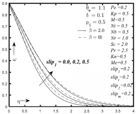
$\omega(\eta)=1+\operatorname{slip}_{m} \omega^{\prime}(\eta);$
$\eta \rightarrow \infty:$
$f^{\prime}(\eta) \rightarrow 0, \theta(\eta) \rightarrow 0, \phi(\eta) \rightarrow 0$ (12)
where, $\operatorname{Slip}_{1}=L_{1} \sqrt{\frac{a}{v}}$; first order slip velocity $\operatorname{Slip}_{2}=L_{1} \sqrt{\frac{a}{v}}$; second order slipparameter $\operatorname{Slip}_{3}=L_{1} \sqrt{\frac{a}{v}}$, parameter of temperature slip, $R=\frac{4 \sigma T_{\infty}^{3}}{k_{\infty} k^{*}}$; parameter of Radiation, K*; thermal radiation parameter, $M=\frac{\sigma B_{0}^{2}}{a p}$: parameter of Magnetic field, $K_{n}=\frac{k_{n}}{a}\left(C_{w}-C_{\infty}\right)^{n-1}$: parameter of chemical reaction, $\delta=\frac{Q}{a(\rho c)_{f}}$; δ< 0 refers to heat generationand δ < 0 represents heat absorption parameters, $\theta_{w}=\frac{T_{w}}{T_{\infty}}$: parameter of temperature difference, $N_{t}=\frac{(\rho c)_{p} D_{T}\left(T_{W}-T_{\infty}\right)}{v T_{\infty}(\rho c)_{f}}$ parameter of: thermophoresis $N_{b}=\frac{(\rho c)_{p} D_{B} C_{\infty}}{v(\rho c)_{f}}$; parameter of Brownian motion, $S C=\frac{v}{D_{B}}$: Schmidt number of mass.
The local Sherwood, Nusselt, density number, and coefficients of skin friction Sh, Nux, Nnx, Cf, are given as follows:
$\begin{aligned} S h &=\frac{r J_{w}}{D_{B}\left(C_{w}-C_{\infty}\right)}, N u_{r}=\frac{r q_{w}}{k\left(T_{w}-T_{\infty}\right)} \text { and } \\ C_{f} &=\frac{\tau_{w}}{\rho U_{w}^{2}} \end{aligned},$ (13)
$\tau_{w}=\left.\mu_{0}\left(1+\frac{1}{\beta}\right) \frac{\partial^{2} u}{\partial z^{2}}\right|_{z=0}, q_{w}=-k\left(\frac{\partial T}{\partial z}\right)+\left.\left(q_{r}\right)\right|_{z=0};$
$J_{w}=-D_{B}\left(\frac{\partial C}{\partial z}\right)_{z=0}, M_{w}=-D_{n}\left(\frac{\partial N}{\partial z}\right)_{z=0}$ (14)
$C_{f} \operatorname{Re}^{\frac{1}{2}}=\left.\left(1+\frac{1}{\beta}\right) f^{\prime \prime}(0)\right|_{\eta=0}$ (15)
$N u \mathrm{Re}^{\frac{-1}{2}}=-\left(1+\frac{4 R}{3}\left\{1+\left(\theta_{w}-1\right) \theta(0)\right\}^{3}\right) \theta^{\prime}(0)$ (16)
$S h \mathrm{Re}^{\frac{-1}{2}}=-\phi^{\prime}(0)$ (17)
$N n \mathrm{Re}^{\frac{-1}{2}}=-\omega^{\prime}(0)$ (18)
$R e=\frac{r u_{w}}{V}$: local Reynolds number.
Utilizing Matlab inbuilt tool bvp4c the numerical solution of Eqns. (8-9) equipped with boundary condition (12) are computed. Applying various values of required parameters given computations are carried out with the aid of graphical data. Blowbackcs of the concerning parameters related to temperature, velocity and mass profiles are analyzed. These physical parameters are employed in the following endurable ranges 0 ≤ M ≤ 1, 0 ≤ Kp ≤ 1,0.8 ≤ b ≤ 5, 0 ≤ Me ≤ 2, 0 ≤ slip1 ≤0.5, 0 ≤ slip2 ≤0.2, 0 ≤ slipt ≤0.2, 0 ≤ R ≤ 2.0, 2.0 ≤ Pr ≤ 3.0, 0.5 ≤ Nt ≤ 0.7,2.0 ≤Sc ≤ 3.0, 2.0 ≤ Sc ≤ 0.7, 0.2 ≤ Pe ≤ 0.4, 2.0 ≤ Sn ≤ 3.0.Therefore the analysis is carried out by varying the following parameters one by one all over the graphical representation n=0.5, We=0.5,Nt=0.5, R = 1.0, Sc=2.0, Pr=2.5, w = 1.1, Nb=0.5, Q = 0.03, Kn=0.5, Me=1.0, slip1 =0.5, slipt =0.5, slip2 =0.2, M=0.5. Furthermore these are considered as fix parameters.
A comparative investigation is performed for the affirmation of available numerical prosaic with already established results. Our computed result of Cf,Nux, Sh for many values of M is correlated to those indicated by Rehman et al. [30], Khan et al. [31] and Nadeem et al. [32] (Table 1-2). We observed that our computed results exhibit outstanding influences with Makinde, Azam, Ramzan.
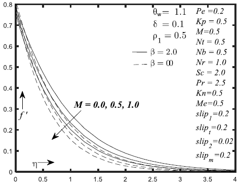
Figure 1. Velocity effect for alteration in M
Figure 2. Temperature effect for alteration in M
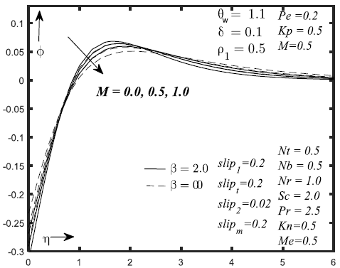
Figure 3. Concentration effect for alteration in M
Figure 4. Influence of M on micro-organism boundary layer
Figure 5. Velocity effect for alteration in Kp
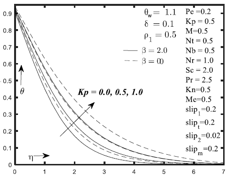
Figure 6. Temperature effect for alteration in Kp
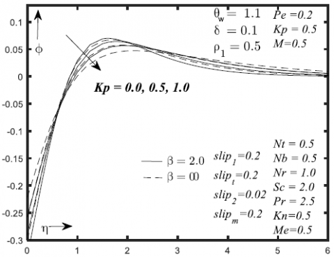
Figure 7. Concentration effect for alteration in Kp
Figure 8. Micro-organism effect for alteration in Kp
Figures 1-4 depicts the variations of involved physical parameters on the f ', θ, ϕ and ω profiles. Figure 1 & 3 reflects the difference in the values of f ' and ϕ with respect to parameter M. This figure depicts that f ' and ϕ decreases when M is increasing. The influence of M parameter on the θ and ω profiles are exhibit in Figures 2 & 4. By improving M, raises θ profile whereas the opposite behaviour is observed on ω profile. Figures 5-8 demonstrate the effect of the kp on f ', θ, ϕ, ω profiles. Variation of f ' and ϕ with respect to Kp parameter is presented in Figures 5 & 7. This figure depicts that f ' and ϕ decreases when Kp is increasing. Figures 6 & 8 outline the consequences of Kp parameter on the θ and ω profiles. Expanding Kp governs gain in θ profile whereas the opposite behavior is observed on ω profile.
Figure 9. Velocity effect for alteration in β
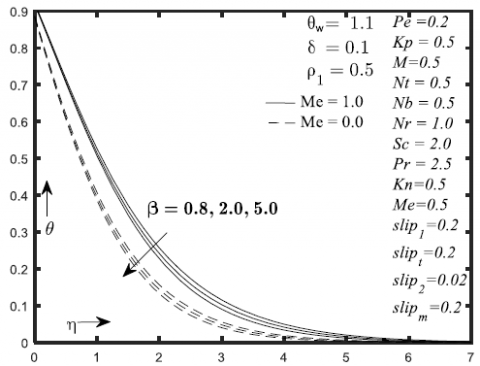
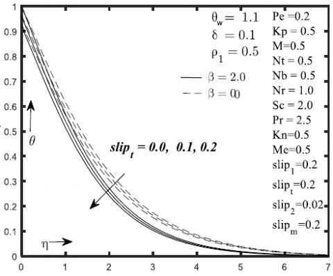
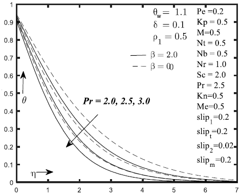
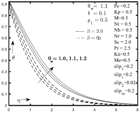
Figure 10. Temperature effect for alteration in β
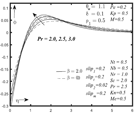
Figure 11. Concentration effect for alteration in β
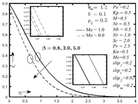
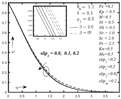
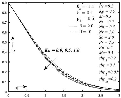
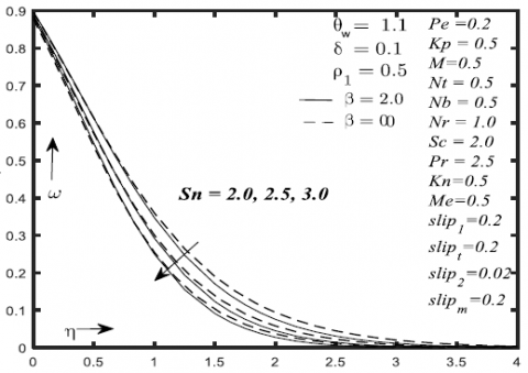
Figure 12. Micro-organism effect for alteration in β
Figure 13. Velocity effect for alteration in Me
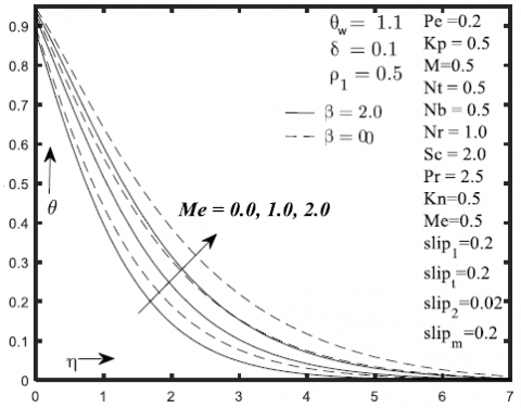
Figure 14. Temperature effect for alteration in Me
Figure 15. Concentration effect for alteration in Me
Figure 16. Micro-organism effect for alteration in Me
Figures 9-12 represent the prominences of β on f', θ, ϕ and ω profiles are drafted in. When the values of β is increased the f', θ, ϕ and ω profiles gets cut down whereas concentration profile is boosted. Figures 13-16 reflects the variations of Me on the f', θ, ϕ and ω profiles. The variation of f', θ and ω profiles with respect to Me parameter is presented in Figure 13, 14 & 16. This figure depicts that the f', θ and ω profiles are boosted when Me parameter is increasing. Figure 15 shows the effect of Me parameter on ϕ profile. Increased value of Me results in suppression of ϕ profile.
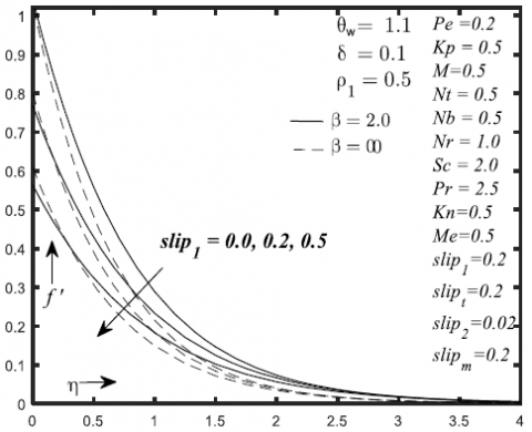
Figure 17. Velocity effect for alteration in slip1
Figure 18. Temperature effect for alteration in slip1
Figure 19. Concentration effect for alteration in slip1
Figure 20. Micro-organism effect for alteration in slip1
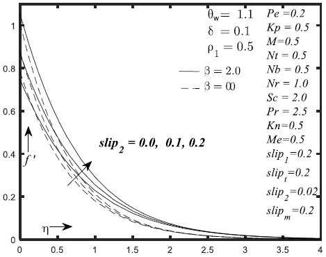
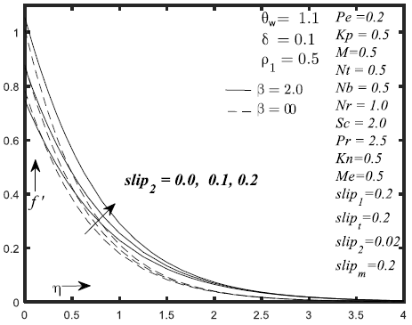
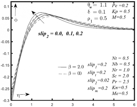
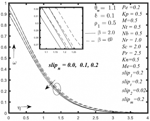
The impact of parameter (slip1) on f', θ, ϕ and ω distributions are drafted in Figures 17-20. To bring the development in parameter (slip1), f' together with ϕ distributions decreases whereas θ, and ω profiles are improved. Figures 21- 24 show the variation of (slip2) on the f ', θ, ϕ and ω profiles. This figure depicts that the f', θ and ϕ profiles are boosted with the expansion of parameter (slip2). The impact of parameter (slipt) on θ, ϕ and ω distributions are drafted in Figures 25 -27. Boost in the parameter of (slipt), results in the decline of θ, ϕ and ω distributions. The effect of (slipm), on the ω distributions is studied in Figure 28. Here an increase in (slipm) results the decreases in ω distributions.
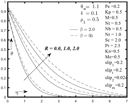
The contrasts of R on θ, ϕ and ω distributions are established in Figures 29-31. The expansion in values of parameter R results the increase in θ profile whereas the reverse observation is shown on ϕ and ω distributions.
The effect of Pr on the θ, ϕ and ω distributions are studied in Figure 32-34. By improving Pr, θ and ω profile gets cut down whereas the opposite behavior is reflected on ϕ distribution.
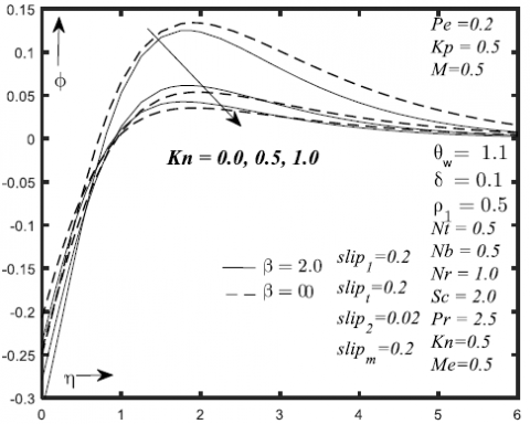
The effect of temperature ratio θw on the θ, ϕ and ω distributions are studied in Figures 35-37. Here an increase in θw observes the increase in the θ distributions whereas the opposite behavior is shown on ϕ and ω distributions. To observe the impact of the parameter Kn on ϕ and ω profiles Figure 38-39 are studied It is analysed that increased values Kn, ϕ and ω profiles gets cut down.
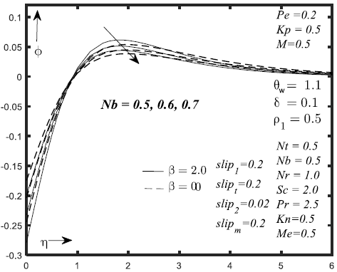
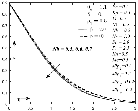
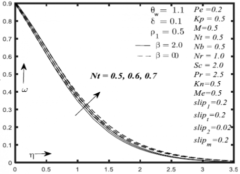
Figure 40-41 represent the effect of Nb on the ϕ and ω distributions. Here an increase in Nb decreases the ϕ and ω profiles. Physically, the Brownian motion expansion aids to tepid the boundary surface which outcomes to passage the nano-particles from the stretching sheet to the fluid in order to reduce the concentration. The effect of Nt on the ϕ and ω distributions are studied in Figure 42-43. Here an increase in Nt increases the ϕ and ω profiles.
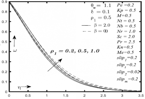
Figure 44 is displayed in order to explore the effect of the Sc on ϕ profile. by improving Sc, ϕ profile gets cuts down when the values of the Sc parameter are increased. Physically, the mass flux of the fluid gets declined as a consequence of improving Sc parameter. The mass flux of fluid gets weaken with the species diffusion by this principle and Sc is observed to be proportional to the diffusion coefficient. Figure 45 demonstrate the effect of Sn parameter on ω profile. When the values of the Sn parameter are hiked, the ω profile gets depleted. The effect of the Pe and ρ1 parameters on ω profile are represented in the Figures 46-47. show the influence of Pe, ρ1 on ω profile. It is discovered that when the values of the parameter Pe and ρ1 are enhanced, the microorganism profile gets depressed.
Table 1-2 represents impact of numerous physical parameters on coefficient of skin friction $C_{f} R e_{x}^{\frac{1}{2}}$, local Nusselt number $N_{u} R e_{x}^{\frac{1}{2}}$ and local Sherwood number $\operatorname{Sh} R e^{\frac{1}{2}}$ with or without melting surface. Table (3-4) reflects the comparative investigation with those given by Rehman et al. [30], Khan et al. [31] and Nadeem et al. [32]. In some limiting cases the given results have an excellent collaboration with those already available results.
Figure 21. Velocity effect for alteration in slip2
Figure 22. Temperature effect for alteration in slip2
Figure 23. Concentration effect for alteration in slip2
Figure 24. Micro-organism effect for alteration in slip2
Figure 25. Temperature effect for alteration in slipt
Figure 26. Concentration effect for alteration in slipt
Figure 27. Micro-organism effect for alteration in slipn
Figure 28. Micro-organism effect for alteration in slipn
Figure 29. Temperature effect for alteration in R
Figure 30. Concentration effect for alteration in R
Figure 31. Micro-organism effect for alteration in R
Figure 32. Temperature effect for alteration in Pr
Figure 33. Concentration effect for alteration in Pr
Figure 34. Micro-organism effect for alteration in Pr
Figure 35. Temperature effect for alteration in θw
Figure 36. Concentration effect for alteration in θw
Figure 37. Micro-organism effect for alteration in θw
Figure 38. Concentration effect for alteration in Kn
Figure 39. Micro-organism effect for alteration in Kn
Figure 40. Concentration effect for alteration in Nb
Figure 41. Micro-organism effect for alteration in Nb
Figure 42. Concentration effect for alteration in Nt
Figure 43. Micro-organism effect for alteration in Nt
Figure 44. Concentration effect for alteration in Sc
Figure 45. Micro-organism effect for alteration in Sn
Figure 46. Micro-organism effect for alteration in Pe
Figure 47. Micro-organism effect for alteration in r1
Table 1. The skin friction coefficient $C_{f} R e_{x}^{\frac{1}{2}}$, local Nusselt number $N u R e_{x}^{\frac{-1}{2}}$ and local Sherwood number $\operatorname{Sh} R e^{\frac{-1}{2}}$ and local density number of the motile microorganisms Nnx are following physically parameter with Casson fluid
|
M |
Kp |
b |
Me |
Slip1 |
Slip2 |
$C_{f} R e_{x}^{\frac{1}{2}}$
|
$N u R e_{x}^{\frac{-1}{2}}$
|
$\operatorname{Sh} R e^{\frac{-1}{2}}$ |
$\mathrm{Nn} R e^{\frac{-1}{2}}$ |
|
0.0 |
|
|
|
|
|
-1.161403085 |
1.203269385 |
-0.440374287 |
0.527625972 |
|
0.5 |
|
|
|
|
|
-1.302302686 |
1.099529430 |
-0.401867531 |
0.519943760 |
|
1.0 |
|
|
|
|
|
-1.426987856 |
1.005109265 |
-0.366910399 |
0.515284155 |
|
|
0.0 |
|
|
|
|
-1.091049200 |
1.263770361 |
-0.462879538 |
0.534109320 |
|
|
0.5 |
|
|
|
|
-1.302302686 |
1.099529430 |
-0.401867531 |
0.519943760 |
|
|
1.0 |
|
|
|
|
-1.475620550 |
0.955872033 |
-0.348715281 |
0.512968956 |
|
|
|
0.8 |
|
|
|
-1.611455729 |
1.111792588 |
-0.406414014 |
0.508053427 |
|
|
|
2 |
|
|
|
-1.302302686 |
1.099529430 |
-0.401867531 |
0.519943760 |
|
|
|
5 |
|
|
|
-1.158969332 |
1.074879436 |
-0.392733100 |
0.525065072 |
|
|
|
|
0.0 |
|
|
-1.394125580 |
1.564257875 |
-0.575185967 |
0.721663808 |
|
|
|
|
1.0 |
|
|
-1.302302686 |
1.099529430 |
-0.401867531 |
0.519943760 |
|
|
|
|
2.0 |
|
|
-1.254955194 |
0.849582889 |
-0.309516194 |
0.421096436 |
|
|
|
|
|
0.0 |
|
-1.874791939 |
1.385229952 |
-0.508168005 |
0.584703773 |
|
|
|
|
|
0.2 |
|
-1.302302686 |
1.099529430 |
-0.401867531 |
0.519943760 |
|
|
|
|
|
0.5 |
|
-0.912584374 |
0.820910201 |
-0.298960226 |
0.473072714 |
|
|
|
|
|
|
0.0 |
-1.260795628 |
1.074158925 |
-0.392466192 |
0.514957659 |
|
|
|
|
|
|
0.1 |
-1.505375405 |
1.213027293 |
-0.444001644 |
0.543859310 |
|
|
|
|
|
|
0.2 |
-1.901212027 |
1.396239511 |
-0.512280260 |
0.587484565 |
Table 2. The skin friction coefficient $C_{f} R e_{x}^{\frac{1}{2}}$, local Nusselt number $N u R e_{x}^{\frac{-1}{2}}$ and local Sherwood number $\operatorname{Sh} R e^{\frac{-1}{2}}$ and local density number of the motile microorganisms Nnx are following physically parameter without Casson fluid
|
M |
Kp |
b |
Me |
Slip1 |
Slip2 |
$C_{f} R e_{x}^{\frac{1}{2}}$ |
$N u R e^{\frac{-1}{2}}$ |
$\operatorname{Sh} R e^{\frac{-1}{2}}$ |
$\mathrm{Nn} R e^{\frac{-1}{2}}$ |
|
0.0 |
|
|
|
|
|
-0.985830427 |
1.103850556 |
-0.403469393 |
0.531321032 |
|
0.5 |
|
|
|
|
|
-1.109280125 |
0.982726198 |
-0.358636085 |
0.525669351 |
|
1.0 |
|
|
|
|
|
-1.218364801 |
0.874825284 |
-0.318815755 |
0.523047831 |
|
|
0.0 |
|
|
|
|
-0.921938390 |
1.172888879 |
-0.429086702 |
0.536529620 |
|
|
0.5 |
|
|
|
|
-1.109280125 |
0.982726198 |
-0.358636085 |
0.525669351 |
|
|
1.0 |
|
|
|
|
-1.263306252 |
0.821854160 |
-0.299307624 |
0.521994361 |
|
|
|
0.8 |
|
|
|
-1.691998945 |
1.583589262 |
-0.582441489 |
0.713536357 |
|
|
|
2 |
|
|
|
-1.394125580 |
1.564257875 |
-0.575185967 |
0.721663808 |
|
|
|
5 |
|
|
|
-1.254672706 |
1.531840350 |
-0.563027222 |
0.721737301 |
|
|
|
|
0.0 |
|
|
-1.199751377 |
1.430406273 |
-0.525049694 |
0.708029256 |
|
|
|
|
1.0 |
|
|
-1.109280125 |
0.982726198 |
-0.358636085 |
0.525669351 |
|
|
|
|
2.0 |
|
|
-1.064986159 |
0.747991514 |
-0.272150042 |
0.438627642 |
|
|
|
|
|
0.0 |
|
-1.495619223 |
1.224749610 |
-0.448360463 |
0.573502728 |
|
|
|
|
|
0.2 |
|
-1.109280125 |
0.982726198 |
-0.358636085 |
0.525669351 |
|
|
|
|
|
0.5 |
|
-0.813162637 |
0.731374240 |
-0.266047371 |
0.489200151 |
|
|
|
|
|
|
0.0 |
-1.082016392 |
0.962538541 |
-0.351177462 |
0.522230580 |
|
|
|
|
|
|
0.2 |
-1.237135822 |
1.071178147 |
-0.391362037 |
0.541761991 |
|
|
|
|
|
|
0.5 |
-1.461309843 |
1.205984779 |
-0.441383602 |
0.569376930 |
Table 3. The local Nusselt number $N u R e_{x}^{\frac{-1}{2}}$ and local Sherwood number $\operatorname{Sh} R e^{\frac{-1}{2}}$ and local density number of the motile microorganisms Nnx are following physically parameter with Casson fluid
|
R |
Pr |
Tw |
Nb |
Nt |
Slipt |
Slipn |
R |
Pr |
$N u R e_{x}^{\frac{-1}{2}}$ with |
$\operatorname{Sh} R e^{\frac{-1}{2}}$ with |
$N n R e^{\frac{-1}{2}}$ with |
|
1.0 |
|
|
|
|
|
|
|
|
0.6560763 |
-0.6560763 |
0.3086786 |
|
2.0 |
|
|
|
|
|
|
|
|
1.0995294 |
-0.4018675 |
0.5199437 |
|
3.0 |
|
|
|
|
|
|
|
|
1.3172271 |
-0.2931813 |
0.6203868 |
|
|
2.0 |
|
|
|
|
|
|
|
0.9017537 |
-0.3287431 |
0.5358111 |
|
|
2.5 |
|
|
|
|
|
|
|
1.0995294 |
-0.4018675 |
0.5199437 |
|
|
3.0 |
|
|
|
|
|
|
|
1.2896108 |
-0.4725025 |
0.5033859 |
|
|
|
1.0 |
|
|
|
|
|
|
1.0251561 |
-0.4393526 |
0.4849680 |
|
|
|
1.1 |
|
|
|
|
|
|
1.0995294 |
-0.4018675 |
0.5199437 |
|
|
|
1.2 |
|
|
|
|
|
|
1.1754801 |
-0.3649500 |
0.5546218 |
|
|
|
|
0.5 |
|
|
|
|
|
1.0995294 |
-0.4018675 |
0.5199437 |
|
|
|
|
1.0 |
|
|
|
|
|
1.0995295 |
-0.2009337 |
0.5779369 |
|
|
|
|
2.0 |
|
|
|
|
|
1.0995302 |
-0.1004669 |
0.6069305 |
|
|
|
|
|
0.5 |
|
|
|
|
1.0995294 |
-0.4018675 |
0.5199437 |
|
|
|
|
|
1.0 |
|
|
|
|
1.2050007 |
-0.8820356 |
0.3512494 |
|
|
|
|
|
2.0 |
|
|
|
|
1.4704564 |
-2.1601303 |
-0.114398 |
|
|
|
|
|
|
0.0 |
|
|
|
1.1795216 |
-0.4251038 |
0.4993342 |
|
|
|
|
|
|
0.1 |
|
|
|
1.1385704 |
-0.4133136 |
0.5097526 |
|
|
|
|
|
|
0.2 |
|
|
|
1.0995294 |
-0.4018675 |
0.5199437 |
|
|
|
|
|
|
|
0.0 |
|
|
1.0995294 |
-0.4018675 |
0.5851888 |
|
|
|
|
|
|
|
0.1 |
|
|
1.0995294 |
-0.4018675 |
0.5506403 |
|
|
|
|
|
|
|
0.2 |
|
|
1.0995294 |
-0.4018675 |
0.5199437 |
|
|
|
|
|
|
|
|
0.0 |
|
0.6560763 |
-0.6560763 |
0.3086786 |
|
|
|
|
|
|
|
|
1.0 |
|
1.0995294 |
-0.4018675 |
0.5199437 |
|
|
|
|
|
|
|
|
2.0 |
|
1.3172271 |
-0.2931813 |
0.6203868 |
|
|
|
|
|
|
|
|
|
2.5 |
1.0995294 |
-0.4018675 |
0.5199437 |
|
|
|
|
|
|
|
|
|
3.0 |
1.2896108 |
-0.4725025 |
0.5033859 |
|
|
|
|
|
|
|
|
|
4.0 |
1.6513396 |
-0.6078990 |
0.4679589 |
Table 4. The local Nusselt number $N u R e_{x}^{\frac{-1}{2}}$ and local Sherwood number $\operatorname{Sh} R e^{\frac{-1}{2}}$ and local density number of the motile microorganisms Nnx are following physically parameter without Casson fluid
|
R |
Pr |
Tw |
Nb |
Nt |
Slipt |
Slipn |
R |
Pr |
$N u R e^{\frac{-1}{2}}$ with out |
$\operatorname{Sh} R e^{\frac{-1}{2}}$ without |
$N n R e^{\frac{-1}{2}}$ without |
|
1.0 |
|
|
|
|
|
|
|
|
0.6205200 |
-0.6205200 |
0.2954334 |
|
2.0 |
|
|
|
|
|
|
|
|
0.9827261 |
-0.3586360 |
0.5256693 |
|
3.0 |
|
|
|
|
|
|
|
|
1.1421394 |
-0.2537846 |
0.6268930 |
|
|
2.0 |
|
|
|
|
|
|
|
0.7904240 |
-0.2877451 |
0.5469702 |
|
|
2.5 |
|
|
|
|
|
|
|
0.9827261 |
-0.3586360 |
0.5256693 |
|
|
3.0 |
|
|
|
|
|
|
|
1.1728880 |
-0.4290864 |
0.5039057 |
|
|
|
1.0 |
|
|
|
|
|
|
0.9787603 |
-0.4194687 |
0.4931733 |
|
|
|
1.1 |
|
|
|
|
|
|
1.0451960 |
-0.3817412 |
0.5287097 |
|
|
|
1.2 |
|
|
|
|
|
|
1.1116979 |
-0.3446591 |
0.5638711 |
|
|
|
|
0.5 |
|
|
|
|
|
1.0451960 |
-0.3817412 |
0.5287097 |
|
|
|
|
1.0 |
|
|
|
|
|
1.0451962 |
-0.1908706 |
0.5859173 |
|
|
|
|
2.0 |
|
|
|
|
|
1.0451962 |
-0.0954353 |
0.6144701 |
|
|
|
|
|
0.5 |
|
|
|
|
1.0451960 |
-0.3817412 |
0.5287097 |
|
|
|
|
|
1.0 |
|
|
|
|
1.1397659 |
-0.8335807 |
0.3660185 |
|
|
|
|
|
2.0 |
|
|
|
|
1.3720788 |
-2.0130296 |
-0.076422 |
|
|
|
|
|
|
0.0 |
|
|
|
1.1160524 |
-0.4022293 |
0.5101668 |
|
|
|
|
|
|
0.1 |
|
|
|
1.0798604 |
-0.3918545 |
0.5195286 |
|
|
|
|
|
|
0.2 |
|
|
|
1.0451960 |
-0.3817412 |
0.5287097 |
|
|
|
|
|
|
|
0.0 |
|
|
1.0995294 |
-0.4018675 |
0.5851888 |
|
|
|
|
|
|
|
0.1 |
|
|
1.0995294 |
-0.4018675 |
0.5506403 |
|
|
|
|
|
|
|
0.2 |
|
|
1.0995294 |
-0.4018675 |
0.5199437 |
|
|
|
|
|
|
|
|
0.0 |
|
0.6484697 |
-0.6484697 |
0.3032480 |
|
|
|
|
|
|
|
|
1.0 |
|
1.0451960 |
-0.3817412 |
0.5287097 |
|
|
|
|
|
|
|
|
2.0 |
|
1.2229232 |
-0.2719453 |
0.6316321 |
|
|
|
|
|
|
|
|
|
2.5 |
1.0451960 |
-0.3817412 |
0.5287097 |
|
|
|
|
|
|
|
|
|
3.0 |
1.2386585 |
-0.4535340 |
0.5086112 |
|
|
|
|
|
|
|
|
|
4.0 |
1.6090186 |
-0.5919913 |
0.4678370 |
Table 5. Comparison of -θ'(0) for various values Pr when Me=Kp=R=Nb=0, Sip1= Sip2 =Nt=M=$\delta$ =0, $\theta_{\mathrm{W}}$=1 and $\beta \rightarrow \infty$
|
Pr |
Nadeem et al. [33] |
Khan et al. [34] |
Golra et al. [35] |
Wang [36] |
Narayana et al. [37] |
Present study |
|
0.7 |
0.454 |
0.454 |
0.454 |
0.454 |
0.4539 |
0.454049257 |
|
2.0 |
0.911 |
0.911 |
0.911 |
0.911 |
0.9114 |
0.911360664 |
Table 6. Comparison of - f ''(0) for various values M when Me=Kp=R=Nb=0, Sip1= Sip2=Nt =$\delta$ =0, $\theta_{\mathrm{W}}$ =1 and $\beta \rightarrow \infty$
|
M |
Anderson et al. [38] |
Prasad et al. [39] |
Mukhopadhyay et al. [40] |
Palani et al. [41] |
Present study |
|
0.0 |
1.000000 |
1.000174 |
1.000173 |
1.00000 |
1.000001171 |
|
0.5 |
1.224900 |
1.224753 |
1.224753 |
1.224745 |
1.224744873 |
|
1 |
1.414000 |
1.414449 |
1.414450 |
1.414214 |
1.414213562 |
|
1.5 |
1.581000 |
1.581139 |
1.581140 |
1.581139 |
1.581138830 |
|
2 |
1.732000 |
1.732203 |
1.732203 |
1.732051 |
1.732050808 |
Table 5 and Table 6 are the comparison table of -θ(0) and -f''(0).
The steady boundary layer flow of Casson nanofluid over a radially surface with zero mass flux, nonlinear radiation and temperature jump has been numerically investigated. Using the pictorial representations the upshot of numerous parameters on velocity, temperature and nanoparticles mass field, are examined. The in cooperation of tabulated numerically computed value along with requisite discussions to the analyzed problem is also reflected.
After oversight the complete study the main conclusion are emerging as follows:
The f', f, θ profiles are boosted with the expansion of parameter (slip2), whereas ω profile is get cut down.
[1] Rehman, K.U., Malik, M.Y., Zahri, M., Tahir, M. (2018). Numerical analysis of MHD Casson Navier’s slip nanofluid flow yield by rigid rotating disk. Results in Physics, 8: 744-751. https://doi.org/10.1016/j.rinp.2018.01.017
[2] Rehman, K.U., Malik, A.A., Malik, M.Y., Sandeep, N., Saba, N.U. (2017). Numerical study of double stratification in Casson fluid flow in the presence of mixed convection and chemical reaction. Results in Physics, 7: 2997-3006. https://doi.org/10.1016/j.rinp.2017.08.020
[3] Mustafa, M., Hayat, T., Pop, I., Aziz, A. (2011). Unsteady boundary layer flow of a Casson fluid due to an impulsively started moving flat plate. Heat Transfer—Asian Research, 40(6): 563-576. https://doi.org/10.1002/htj.20358
[4] Nadeem, S., Haq, R.U., Lee, C. (2012). MHD flow of a Casson fluid over an exponentially shrinking sheet. Scientia Iranica, 19(6): 1550-1553. https://doi.org/10.1016/j.scient.2012.10.021
[5] Mukhopadhyay, S. (2013). Casson fluid flow and heat transfer over a nonlinearly stretching surface. Chinese Physics B, 22(7): 074701. https://doi.org/10.1088/1674-1056/22/7/074701
[6] Mukhopadhyay, S., Moindal, I.C., Hayat, T. (2014). MHD boundary layer flow of Casson fluid passing through an exponentially stretching permeable surface with thermal radiation. Chinese Physics B, 23(10): 104701. https://doi.org/10.1088/1674-1056/23/10/104701
[7] Ramesh, K., Devakar, M. (2015). Some analytical solutions for flows of Casson fluid with slip boundary conditions. Ain Shams Engineering Journal, 6(3): 967-975. https://doi.org/10.1016/j.asej.2015.02.007
[8] Mustafa, M., Khan, J.A. (2015). Model for flow of Casson nanofluid past a non-linearly stretching sheet considering magnetic field effects. AIP Advances, 5(7): 077148. https://doi.org/10.1063/1.4927449
[9] Qing, J., Bhatti, M.M., Abbas, M.A., Rashidi, M.M., Ali, M.E.S. (2016). Entropy generation on MHD Casson nanofluid flow over a porous stretching/shrinking surface. Entropy, 18(4): 123. https://doi.org/10.3390/e18040123
[10] Sandeep, N., Koriko, O.K., Animasaun, I.L. (2016). Modified kinematic viscosity model for 3D-Casson fluid flow within boundary layer formed on a surface at absolute zero. Journal of Molecular Liquids, 221: 1197-1206. https://doi.org/10.1016/j.molliq.2016.06.049
[11] Raju, C.S.K., Hoque, M.M., Sivasankar, T. (2017). Radiative flow of Casson fluid over a moving wedge filled with gyrotactic microorganisms. Advanced Powder Technology, 28(2): 575-583. https://doi.org/10.1016/j.apt.2016.10.026
[12] Ali, M.E., Sandeep, N. (2017). Cattaneo-Christov model for radiative heat transfer of magnetohydrodynamic Casson-ferrofluid: a numerical study. Results in Physics, 7: 21-30. https://doi.org/10.1016/j.rinp.2016.11.055
[13] Imtiaz, M., Hayat, T., Alsaedi, A., Asghar, S. (2017). Slip flow by a variable thickness rotating disk subject to magnetohydrodynamics. Results in Physics, 7: 503-509. https://doi.org/10.1016/j.rinp.2016.12.021
[14] Rashidi, M.M., Kavyani, N., Abelman, S. (2014). Investigation of entropy generation in MHD and slip flow over a rotating porous disk with variable properties. International Journal of Heat and Mass Transfer, 70: 892-917. https://doi.org/10.1016/j.ijheatmasstransfer.2013.11.058
[15] Hayat, T., Muhammad, T., Shehzad, S.A., Alsaedi, A. (2017). On magnetohydrodynamic flow of nanofluid due to a rotating disk with slip effect: A numerical study. Computer Methods in Applied Mechanics and Engineering, 315: 467-477. https://doi.org/10.1016/j.cma.2016.11.002
[16] Kumaran, G., Sandeep, N. (2017). Thermophoresis and Brownian moment effects on parabolic flow of MHD Casson and Williamson fluids with cross diffusion. Journal of Molecular Liquids, 233: 262-269. https://doi.org/10.1016/j.molliq.2017.03.031
[17] Rehman, K.U., Qaiser, A., Malik, M.Y., Ali, U. (2017). Numerical communication for MHD thermally stratified dual convection flow of Casson fluid yields by stretching cylinder. Chinese Journal of Physics, 55(4): 1605-1614. https://doi.org/10.1016/j.cjph.2017.05.002
[18] Ahmed, J., Shahzad, A., Khan, M., Ali, R. (2015). A note on convective heat transfer of an MHD Jeffrey fluid over a stretching sheet. AIP Advances, 5(11): 117117.
[19] Shahzad, A., Ali, R. (2012). Approximate analytic solution for magneto-hydrodynamic flow of a non-Newtonian fluid over a vertical stretching sheet. Can J Appl Sci, 2(1): 202-215.
[20] Doh, D.H., Muthtamilselvan, M. (2017). Thermophoretic particle deposition on magnetohydrodynamic flow of micropolar fluid due to a rotating disk. International Journal of Mechanical Sciences, 130: 350-359. https://doi.org/10.1016/j.ijmecsci.2017.06.029
[21] Malik, M.Y., Bilal, S. Bibi, M. (2017). Numerical analysis for MHD thermal and solutal stratified stagnation point flow of Powell-Eyring fluid induced by cylindrical surface with dual convection and heat generation effects. Results in Physics, 7: 482-492. https://doi.org/10.1016/j.rinp.2016.12.025
[22] Turkyilmazoglu, M., Senel, P. (2013). Heat and mass transfer of the flow due to a rotating rough and porous disk. International Journal of Thermal Sciences, 63: 146-158. https://doi.org/10.1016/j.ijthermalsci.2012.07.013
[23] Turkyilmazoglu, M. (2014). Nanofluid flow and heat transfer due to a rotating disk. Computers & Fluids, 94: 139-146. https://doi.org/10.1016/j.compfluid.2014.02.009
[24] Griffiths, P.T., Garrett, S.J., Stephen, S.O. (2014). The neutral curve for stationary disturbances in rotating disk flow for power-law fluids. Journal of Non-Newtonian Fluid Mechanics, 213: 73-81. https://doi.org/10.1016/j.jnnfm.2014.09.009
[25] Mustafa, M., Khan, J.A., Hayat, T., Alsaedi, A. (2015). On Bödewadt flow and heat transfer of nanofluids over a stretching stationary disk. Journal of Molecular Liquids, 211: 119-125. https://doi.org/10.1016/j.molliq.2015.06.065
[26] Sheikholeslami, M., Hatami, M., Ganji, D. D. (2015). Numerical investigation of nanofluid spraying on an inclined rotating disk for cooling process. Journal of Molecular Liquids, 211: 577-583. https://doi.org/10.1016/j.molliq.2015.07.006
[27] Latiff, N.A., Uddin, M.J., Ismail, A.M. (2016). Stefan blowing effect on bioconvective flow of nanofluid over a solid rotating stretchable disk. Propulsion and Power Research, 5(4): 267-278. https://doi.org/10.1016/j.jppr.2016.11.002
[28] Ming, C., Zheng, L., Zhang, X., Liu, F., Anh, V. (2016). Flow and heat transfer of power-law fluid over a rotating disk with generalized diffusion. International Communications in Heat and Mass Transfer, 79: 81-88. https://doi.org/10.1016/j.icheatmasstransfer.2016.10.013
[29] Hayat, T., Rashid, M., Imtiaz, M., Alsaedi, A. (2017). Nanofluid flow due to rotating disk with variable thickness and homogeneous-heterogeneous reactions. International Journal of Heat and Mass Transfer, 113: 96-105. https://doi.org/10.1016/j.ijheatmasstransfer.2017.05.018
[30] Rehman, K.U., Khan, A.A., Malik, M.Y., Pradhan, R.K. (2017). Combined effects of Joule heating and chemical reaction on non-Newtonian fluid in double stratified medium: A numerical study. Results in Physics, 7: 3487-3496. https://doi.org/10.1016/j.rinp.2017.09.003
[31] Khan, I., ur Rehman, K., Malik, M.Y. (2017). Physical aspects of nanoparticles in non-Newtonian liquid in the presence of chemically reactive species through parabolic approach. Results in Physics, 7: 2540-2549. https://doi.org/10.1016/j.rinp.2017.07.027
[32] Nadeem, S., Hussain, S.T. (2014). Flow and heat transfer analysis of Williamson nanofluid. Applied Nanoscience, 4(8): 1005-1012. https://doi.org/10.1007/s13204-013-0282-1
[33] Nadeem, S., Haq, R.U., Akbar, N.S., Khan, Z.H. (2013). MHD three-dimensional Casson fluid flow past a porous linearly stretching sheet. Alexandria Engineering Journal, 52(4): 577-582. https://doi.org/10.1016/j.aej.2013.08.005
[34] Khan, W.A., Pop, I. (2010). Boundary-layer flow of a nanofluid past a stretching sheet. International Journal of Heat and Mass Transfer, 53(11-12): 2477-2483. https://doi.org/10.1007/BF00853952
[35] Gorla, R.S.R., Sidawi, I. (1994). Free convection on a vertical stretching surface with suction and blowing. Applied Scientific Research, 52(3): 247-257. https://doi.org/10.1016/j.ijheatmasstransfer.2010.01.032
[36] Wang, C.Y. (1989). Free convection on a vertical stretching surface. ZAMM‐Journal of Applied Mathematics and Mechanics/Zeitschrift für Angewandte Mathematik und Mechanik, 69(11): 418-420. https://doi.org/10.1002/zamm.19890691115
[37] Narayana, K.L., Gangadhar, K., Subhakar, M.J. (2015). Effect of viscous dissipation on heat transfer of Magneto-Williamson nano fluid. IOSR J Math (IOSR-JM), 11(4): 25-37.
[38] Andersson, H.I., Hansen, O.R., Holmedal, B. (1994). Diffusion of a chemically reactive species from a stretching sheet. International Journal of Heat and Mass Transfer, 37(4): 659-664. https://doi.org/10.1016/0017-9310(94)90137-6
[39] Prasad, K.V., Sujatha, A., Vajravelu, K., Pop, I. (2012). MHD flow and heat transfer of a UCM fluid over a stretching surface with variable thermophysical properties. Meccanica, 47(6): 1425-1439. https://doi.org/10.1007/s11012-011-9526-x
[40] Mukhopadhyay, S., Golam, A.M., Wazed, A.P. (2013). Effects of transpiration on unsteady MHD flow of an UCM fluid passing through a stretching surface in the presence of a first order chemical reaction. Chin Phys B, 22(124701): 1674-1056.
[41] Palani, S., Kumar, B.R., Kameswaran, P.K. (2016). Unsteady MHD flow of an UCM fluid over a stretching surface with higher order chemical reaction. Ain Shams Engineering Journal, 7(1): 399-408. https://doi.org/10.1016/j.asej.2015.11.021