Raghdah W. Saleh*![]() | Hadeel N. Abdullah
| Hadeel N. Abdullah![]()
© 2023 IIETA. This article is published by IIETA and is licensed under the CC BY 4.0 license (http://creativecommons.org/licenses/by/4.0/).
OPEN ACCESS
One type of diabetes is diabetic retinopathy, which results in vascular abnormalities that can result in blindness. Because the effects of this disease are irreversible, early detection is essential because unchecked eye disease can lead to blindness. A crucial first step in automated screening for diabetic retinopathy is the detection of microaneurysms in digital color fundus images. Normal, mild, moderate, severe, and PDR are the five DR stages or grades (proliferative diabetic retinopathy), colored fundus images are often examined by highly qualified specialists to identify this catastrophic condition. Manual diagnosis of this illness (by clinicians) takes time and is error-prone. Numerous computer vision-based methods for automatically identifying DR and its various stages from retina images have so been developed. This study uses fundus-colored images to demonstrate an automated strategy for detecting this condition early and classifying its severity using a convolution neural network.
DR, CNN, BV
The most prevalent condition affecting the eyes is diabetic retinopathy (DR), brought on by the body's excessive blood sugar levels that adversely affect the retina's blood vessels. Effective therapies for DR necessitate early identification and ongoing observation of diabetic patients, but this is a difficult challenge given the disease's delayed onset and lack of symptoms. In America, diabetic retinopathy affects one out of every three diabetes individuals. In contrast, the manual process of performing eye exams takes a lot of time, care, and work. Damage to the retina causes retinopathy, which causes the blood vessels to clog, leak, and develop erratically. As a result., 78% of people over 30 with diabetes who have had it for more than 15 years will develop diabetic retinopathy before it reaches a stage of progression; diabetic retinopathy is asymptomatic and does not damage vision. That results from long-term diabetes mellitus [1, 2]. If DR reaches a severe level, vision loss may result.
DR accounts for 2.6% of blindness globally; the risk of blindness can be decreased by early diagnosis and treatment of DR with regular retinal screening. The primary result of DR is the constriction of the blood vessels in the eyes, to which the eyes have two responses:
The major area (vitreous), which must be clear in order to allow light to get through to the retina—the most sensitive component of the eyes—the rough cornea, pupil, and lens—first sees the creation of new blood vessels and bleeding.
Second, the blood vessels leak, which will have an impact on and destroy the retina, particularly the macula (the central portion of the retina), which is responsible for detailed vision.
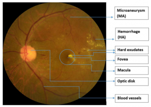
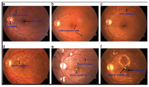
An early stage of diabetic retinopathy is known as non-proliferative diabetic retinopathy [3, 4]. In this stage, the retina's tiny blood veins leak fluid or blood. The fluid leakage causes the retina to enlarge or develop exudates, which are deposits as a result of the retina's blood supply being widely shut off; PDR, or proliferative diabetic retinopathy, is an effort by the eye to construct or replenish the retina's supply of blood vessels (neovascularization) [5]. Figure 1 shows a fundus image with labeled signs of Diabetic Retinopathy.
Figure 1. The main structure of a retina image and DR signs [6]
The earliest indication of DR is microaneurysms (MA), microscopic blood vessel bulges that manifest as dark red dots on the retina because the walls of the blood artery are weak with sharp margins and a dimension of less than 125m. Hemorrhages (HM) are tiny blood discharge patches that appear as more significant spots on the retina when their size exceeds 125m, and they have an asymmetrical edge, while soft exudates (EX) are areas of brilliant yellow color on the retina caused by lipid and protein leaking; they are located in the outer layers of the retina and have angular borders. When nerve fiber swells, hard exudates, often known as cotton wool, develop as brilliant, reflective lesions that look like white patches on the retina. It has an oval or round form. Bright lesions are soft and hard exudates, while red lesions are MA and HM (EX). An ophthalmologist may classify a fundus image as normal or as having a particular level of DR, depending on the existence of DR signals and their complexity [4, 6]; Table 1 illustrates the international clinical diabetic retinopathy severity scales, by executing specific actions referred to as image processing, we can obtain improved photographs. It is frequently employed to identify eye disorders. On the basis of features like blood vessels, hemorrhages, oozes, etc., several techniques for the early detection of DR have been developed. It comprises picture improvement techniques like adaptive histogram equalization for the detection of DR and histogram equalization [7].
Table 1. International clinical diabetic retinopathy severity scales
|
Class |
Findings from Dilated Ophthalmology |
Severity |
|
0 |
Normal |
No DR |
|
1 |
Microaneurysms |
Mild |
|
2 |
Any of followings Microaneurysms and Hemorrhages, hard exudate or cotton wool spots |
Moderate |
|
3 |
More than 20 intra-retinal hemorrhages per quadrant, obvious venous beading in at least two of the quadrants, and substantial intra-retinal micro-vascular abnormality (IRMA) in at least one of the quadrants |
Sever |
|
4 |
Vitreous/pre-retinal hemorrhage Neovascularization |
Proliferative DR |
There has been a lot of study on the identification of diabetic retinopathy using feature extraction models, however, deep learning techniques include notions that are fundamentally distinct from feature extraction techniques that function by autonomously extracting features from a huge number of training images. They frequently recognize particular traits by each hidden layer. Sarfaraz et al. employed a model that had already been trained for a different set of classes that interested us, and we retrained it to assess the severity of diabetic retinopathy in eye photographs (data was provided by eyePacs as color fundus photos via Kaggle). The convolutional neural network classifier with an accuracy of 48.2% for 5-class severity classification was created from the Inception V3 network (trained for ImageNet) [8]. X. Wang et al. used Diabetic Retinopathy (DR) images from Kaggle have been grouped into five groups. For DR stage classification, a number of deep convolutional neural network techniques have been used. InceptionNet V3 has obtained a state-of-the-art accuracy result of 63.23%, demonstrating the efficiency of deploying deep Convolutional Neural Networks for DR image identification [1]. A. Kwasigroch et al. introduced a unique class coding strategy that allowed the objective function being minimized during the training of neural networks to take into account the value of the difference between predicted score and target score. We used quadratic weighted Kappa score, which is calculated between the predicted scores and scores presented in the dataset, to assess the classification performance of the employed models. The most accurate model under test has a detection accuracy of roughly 82% and a stage estimation accuracy of 51%. Additionally, the system attained a respectable Kappa value of 0.776. The outcomes demonstrated that deep learning algorithms can be successfully used to address this incredibly challenging analytical problem [9].
3.1 Dataset
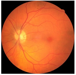
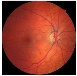
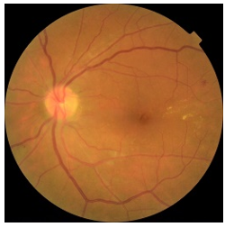
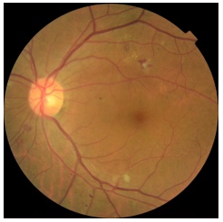
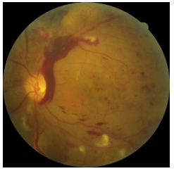
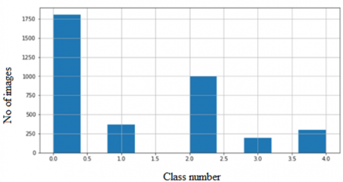
We used 3662 fundus images from Kaggle; every image displayed one of the five different types of DR disease—Normal, Mild, Moderate, Severe, and PDR as shown in Figure 2. Five classes, each divided by training and testing sets, had imbalanced levels, 70% for training and 30% for testing. Figure 3 illustrates the data distribution.
(a)
(b)
(c)
(d)
(e)
Figure 2. Kaggle images of different stages of diabetic retinopathy (a) No DR (b) Mild (c) Moderate (d) Sever
(e) Proliferative DR
Figure 3. Dataset distribution
3.2 Data pre-processing
Each image was pre-processed to remove any background irregularities. Non-uniform light and variations in eye pigment color are two significant causes of this non-uniformity. Before executing the image processing processes, this was rectified by applying adaptive histogram equalization to the image. Image enhancement is an essential part that increases accuracy. In this paper, the pre-processing of the fundus images includes implementing a variety of techniques to get ready for the convolutional layer's feature extraction. Image resizing is part of this preparation. It was resized to 224 × 224 pixels.data imbalance is the most popular problem faced multi class classifications there are many tricks ued for handeling imbalaced dataset we will try to apply any method to improve the poor performance we used the re-weighting method to estimate class weights for unbalanced dataset with balanced from sklearn.utils import class weight also data augmentations another method we have used to solve this problem.
3.3 Data augmentation
The model is overfitting when the number of epochs is unsuitable and the data set used for learning is limited. We employed image augmentation using the following characteristics (Flip vertical and horizontal, Zooming and channel shift) as a crucial procedure for both the training and testing dataset to decrease overfitting and boost the model's accuracy as it is increase the dataset without lossing the information.
3.4 CNN classification model
Convolution neural networks are multi-layer artificial neural networks made especially for handling two-dimensional input data for classifying images. They exhibit strong performance in classifying various supervised learning tasks. Using a set of filters, CNN can extract powerful feature representations from input data layer by layer [10]. It down-samples the data dimension in time and space and combines the sparse connection with the parameter weight-sharing technique. To avoid the algorithm from becoming overfit, it drastically reduces the number of training parameters [11]. For our model, the layers and parameters used were as the following. The input layer for the model started with an image that was 224 x 224 x 3 in size after pre-processing and augmentation. The convolutional layer, Rectified Linear Unit (ReLU), and max-pooling layer are just a few of the numerous layers that these images go through. To avoid overfitting, four dropout layers are used. The sigmoid layer, fully linked layer, and classification layer are the last layers. Additionally, we employ a batch-normalizing layer after the first convolutional layer. The actions of each layer are fully described in the sentences that follow.
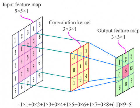
The training data are entered into the model with input size using the input layer 224x 224 x 3. The feature from the input image is extracted using the convolutional layer; this layer contains a kernel filter, which is a filter that has been combined with the input images. It's also important to note that basic image features like lines and edges were extracted from the image using the kernel in the initial layers. While in the advanced layers, significant features are extracted from the kernel. As its output, this layer generates a fresh set of images known as feature maps, where the number of kernels is equal to the number utilized in this layer [12]. In this paper, the number of filters used is 16,16,32,32,64, 64,128, and 128 with kernel size 2 x 2, 3 x 3, 2 x 2, 3 x 3, 3 x 3, 3 x 3, 3 x 3 and 3 x 3 respectively. Figure 4 shows an example of convolution layer operation with kernel size 3 x 3 [13].
Following each convolutional layer comes to an activation function that controls how the connecting node will behave.
Figure 4. Convolutional layer [13]
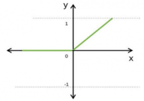
Instead of normalizing the entire data set during pre-processing, the batch normalization layer is utilized during the training processing, which reduces the training time. Our model employs a rectifier linear unit (ReLU), which produces a positive number and a zero as its output ignoring negative, which can effectively prevent gradient and overfitting, Figure 5 illustrates the behavior of this function and below the mathematical representation of it:
$f(x)=\left\{\begin{array}{l}x, x \geq 0 \\ 0, x \leq 0\end{array}\right.$ (1)
Figure 5. Relu behavior [14]
After the convolutional operation, the dimension of the feature maps was lowered using a pooling layer, which reduced the complexity of the CNN. The concept of a pooling layer is comparable to a convolutional layer, which employs the moving filter on the picture to determine the outcome consistent with the kind of pooling layer applied in the model.
We can use the following formula to compute the output size of the feature map.
$H=\frac{h}{s}$ (2)
$W=\frac{W}{S}$ (3)
where, H stands for the output feature map's height, W for the output feature map's width, h for the input feature map's height, w for the input feature map's width, and s for the pooling operation's stride, Figure 6 below illustrate an example of the max-pooling layer with filter size 2 x 2.
Figure 6. Example of max pooling layer [14]
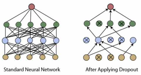
Overfitting is one of the frequent issues with training when the best learning performance is used to compensate for poor testing performance. To avoid overfitting, the dropout layer is frequently used; a percentage value determines the number of nodes in this layer, and some nodes were randomly chosen at specific iterations. The chosen nodes are set to zero, preventing them from impacting the model during training [15]. An example of a dropout layer before and after dropping is shown in Figure 7 below:
Figure 7. Dropout layer [16]
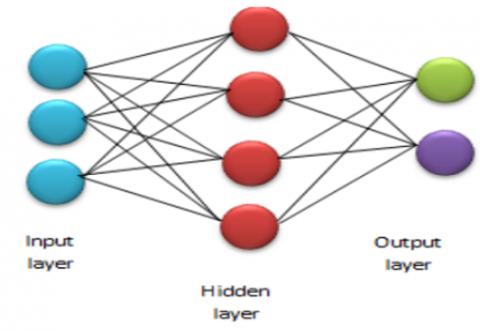
Our proposed model found that the best dropout is 3%, 5%, 3%, and 5%, respectively, for the four dropout layers. The fully connected layer, the sigmoid layer, and the classification layer make up the final three layers. The two-dimensional image is reduced to one dimension using the first (fully connected) layer. Each neuron in this layer is linked to the neuron before it and the neuron after it. This layer produces the same number of categories—five classes—as our model's output. Figure 8 shows an example of a fully connected layer. It should be observed that there is the same number of categories as nodes in this layer, the last layer of ultimately linked layers forecasts the probability result for each category using a unique activation function. Typically, this activation function is a softmax function or, in the case of binary classification as used in our model, a sigmoid function [17].
Figure 8. Fully connected layer [17]
Our proposed model is illustrated in Figure 9 below:
Figure 9. Our proposed model
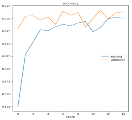
We have used 3662 images from the Kaggle dataset, dividing them into 70% for training and 30% for testing. The primary operations used to prepare the images for the model was image resizing to 224×224×3, employing image augmentation using the following characteristics (Flip vertical and horizontal, Zooming and channel shift) as a crucial procedure should be used for the training and testing datasets. to decrease overfitting and boost the model's accuracy, batch size 32 and Binary crossentropy was utilized as the loss function, ReLU as the activation function, and sigmoid as the activation function in the final layer of the model. Adam was used as the optimizer.We have classified the images into five classes and achieved an accuracy of 71.18%, as shown in Figure 10 below:
Figure 10. Accuracy
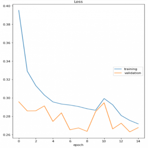
While the loss function is less than 0.3, we must note that the curve first decreases sharply with some oscillations due to the usage of 32 images as a mini-batch size, as shown in Figure 11.
Figure 11. Loss
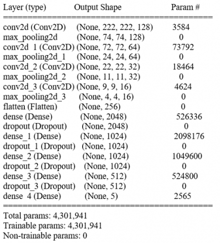
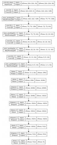
4.1 Hyperparameters and layers of our model:
Various model parameters and the number of layers were tested before the ideal model was found, it is a Keras Sequential API used to define the network. CNNs are defined using the Conv2D layer, our model consists of 18 layers as shown in Figure 13, starting with an input layer (no. of images x dimensions of the image) that receives input images with resolution 224x224 pixels, followed by four convolutional layers(no. of filters x dimensions of a convolved matrix); for feature extraction, a normalization layer for normalizing images, 7 ReLU layers function, Four dropout layers to avoid overfitting, four max-pooling layers to shrink the size of feature maps, a fully connected layer acting as a flatting layer, a sigmoid layer to determine the probability of a class, and then the classification layer to predict the output as shown in Figure 12 below:
Figure 12. Hyperparameters and layers
Figure 13. Proposed sequential model
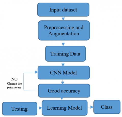
Figure 14 below illustrates the detection of diabetic retinopathy severity from fundus images.
Figure 14. Detection of diabetic retinopathy severity from fundus images
Table 2. Number of neurons and filters used
|
Name of layer |
Image dimensions |
Size of filters |
No. of filters |
No. of neurons |
|
Conv |
224×224 |
3×3 |
128 |
222×222×128=6308352 |
|
Max pooling |
222×222 |
3×3 |
128 |
74×74×128=700928 |
|
Conv_1 |
74×74 |
3×3 |
64 |
72×72×64=331776 |
|
Max pooling _1 |
72×72 |
3×3 |
64 |
24×24×64=36864 |
|
Conv_2 |
24×24 |
3×3 |
32 |
22×22×32=15488 |
|
Max pooling _2 |
22×22 |
2×2 |
32 |
11×11×32=3872 |
|
Conv_3 |
11×11 |
3×3 |
16 |
9×9×16=1296 |
|
Max pooling _3 |
9×9 |
2×2 |
16 |
4×4×16=256 |
The number of neurons and filters that used in our models is illustrated in Table 2.
We made a comparison between previous studies and our proposed work in terms of datasets and method used, and several classes with accuracy achieved noted that 67% was the highest in previous studies [18] as shown below in Table 3:
Table 3. Comparison between previous studies with proposed work
|
Reference |
Source of dataset |
Method |
No. of classes |
Accuracy |
|
[8] |
Kaggle |
CNN |
Five |
48.2% |
|
[1] |
Kaggle |
InceptionV3 |
Five |
63.23% |
|
[9] |
Kaggle |
CNN |
Five |
51% |
|
[18] |
Kaggle |
CNN |
Five |
67% |
|
Proposed |
Kaggle |
CNN |
Five |
71.18% |
This study developed a CNN-based classification model for diabetic retinopathy to group fundus images into five classes: normal eye, mild, moderate, severe, and proliferative DR. our proposed model has 18 layers, starting with an input layer that receives input images, followed by four convolutional layers for feature extraction, a normalization layer for normalizing images, 7 ReLU layers function, Four dropout layers to avoid overfitting, four max-pooling layers to shrink the size of feature maps, a fully connected layer acting as a flatting layer, a sigmoid layer to determine the probability of a class, and then the classification layer to predict the output.
Additionally, data augmentation and pre-processing enabled our model to demonstrate greater accuracy. Up to 70% of the proposed model's predictions are accurate. Additionally, we gave a comparison between the models to demonstrate our model's superiority to the others.
Future efforts could focus on a variety of areas.
First, more sophisticated CNN-based image classification models could be used to increase the accuracy of DR categorization.
Second, approaches for blood vessel and object detection based on CNN could be used to help with DR stage image recognition.
Third, using real-time datasets for detecting retinopathy may be more effective. also we can use 20D Lens and smart phone to capture retina image from a patient and use it.
[1] Wang, X., Lu, Y., Wang, Y., Chen, W.B. (2018). Diabetic retinopathy stage classification using convolutional neural networks. In 2018 IEEE International Conference on Information Reuse and Integration (IRI), pp. 465-471. https://doi.org/10.1109/IRI.2018.00074
[2] Nawaz, F., Ramzan, M., Mehmood, K., Khan, H.U., Khan, S.H., Bhutta, M.R. (2021). Early detection of diabetic retinopathy using machine intelligence through deep transfer and representational learning. CMC Comput. Mater. Contin, 66(2): 1631-1645. http://dx.doi.org/10.32604/cmc.2020.012887
[3] Chun, B.Y., Rizzo III, J.F. (2016). Dominant optic atrophy: Updates on the pathophysiology and clinical manifestations of the optic atrophy 1 mutation. Current Opinion in Ophthalmology, 27(6): 475-480. https://doi.org/10.1097/ICU.0000000000000314
[4] Alyoubi, W.L., Shalash, W.M., Abulkhair, M.F. (2020). Diabetic retinopathy detection through deep learning techniques: A review. Informatics in Medicine Unlocked, 20: 100377. https://doi.org/10.1016/j.imu.2020.100377
[5] Priya, R., Aruna, P. (2013). Diagnosis of diabetic retinopathy using machine learning techniques. ICTACT Journal on Soft Computing, 3(4): 563-575.
[6] Vo, H.H., Verma, A. (2016). New deep neural nets for fine-grained diabetic retinopathy recognition on hybrid color space. In 2016 IEEE International Symposium on Multimedia (ISM), pp. 209-215. https://doi.org/10.1109/ISM.2016.0049
[7] Naveen, R., Sivakumar, S.A., Shankar, B.M., Priyaa, A.K. (2019). Diabetic retinopathy detection using image processing. Int. J. Eng. Adv. Technol, 8(6): 937-941. https://doi.org/10.35940/ijeat.F1179.0886S19
[8] Masood, S., Luthra, T., Sundriyal, H., Ahmed, M. (2017). Identification of diabetic retinopathy in eye images using transfer learning. In 2017 International Conference on Computing, Communication and Automation (ICCCA), pp. 1183-1187. https://doi.org/10.1109/CCAA.2017.8229977
[9] Kwasigroch, A., Jarzembinski, B., Grochowski, M. (2018). Deep CNN based decision support system for detection and assessing the stage of diabetic retinopathy. In 2018 International Interdisciplinary PhD Workshop (IIPhDW), pp. 111-116. https://doi.org/10.1109/IIPHDW.2018.8388337
[10] Zhang, W., Li, C., Peng, G., Chen, Y., Zhang, Z. (2018). A deep convolutional neural network with new training methods for bearing fault diagnosis under noisy environment and different working load. Mechanical Systems and Signal Processing, 100: 439-453. https://doi.org/10.1016/j.ymssp.2017.06.022
[11] Bengio, Y., LeCun, Y. (2007). Scaling learning algorithms towards AI. Large-Scale Kernel Machines, 34(5): 1-41.
[12] Kim, P. (2017). Convolutional neural network. In MATLAB Deep Learning, pp. 121-147. Apress, Berkeley, CA.
[13] Gong, W., Chen, H., Zhang, Z., Zhang, M., Wang, R., Guan, C., Wang, Q. (2019). A novel deep learning method for intelligent fault diagnosis of rotating machinery based on improved CNN-SVM and multichannel data fusion. Sensors, 19(7): 1693. https://doi.org/10.3390/s19071693
[14] Sadoon, T.A., Ali, M.H. (2021). Deep learning model for glioma, meningioma and pituitary classification. Int J Adv Appl Sci., 2252(8814): 8814. https://doi.org/10.11591/IJAAS.V10.I1.PP88-98
[15] Srivastava, N., Hinton, G., Krizhevsky, A., Sutskever, I., Salakhutdinov, R. (2014). Dropout: A simple way to prevent neural networks from overfitting. The Journal of Machine Learning Research, 15(1): 1929-1958.
[16] HUDA SALEH, “Building Convolution Neural Networks For Digit Recognition,” [Online]. Available: https://www.kaggle.com/code/hudasaleh1/cnn-using-keras, accessed on Jan. 17, 2022.
[17] Ghosh, A., Sufian, A., Sultana, F., Chakrabarti, A., De, D. (2020). Fundamental concepts of convolutional neural network. In: Balas, V., Kumar, R., Srivastava, R. (eds) Recent Trends and Advances in Artificial Intelligence and Internet of Things. Intelligent Systems Reference Library, vol 172. Springer, Cham. https://doi.org/10.1007/978-3-030-32644-9_36
[18] Al-Kamachy, I.M.R.K. (2019). Classification of diabetic retinopathy using pre-trained deep learning models. Master's thesis.