Arif Setiawan* | Hadiyanto Hadiyanto | Catur E. Widodo
© 2022 IIETA. This article is published by IIETA and is licensed under the CC BY 4.0 license (http://creativecommons.org/licenses/by/4.0/).
OPEN ACCESS
Shrimp is a marine culture found globally due to the ability of its yields to boost a country's economy. It is imperative to monitor its size to determine the condition of the shrimp underwater with complex noise using a non-invasive method. Therefore, this study aims to develop a new method for measuring the body weight of shrimp using morphometric features based on underwater image analysis and a machine learning approach. The method used consists of several steps, data collection using an underwater camera, image analysis using image grayscale, image binary, edge detection, region of interest detection, shrimp image morphometric features extraction, camera calibration using Triangle Similarity (TS), and Correction Factor (CF), calculation of morphometric features value, create machine learning model, training data, and testing data for estimation of underwater shrimp body weight. After testing the model, get the best accuracy value is RMSE = 0.05, MAE = 0.04, and R2 = 0.96 from the MLR method. In conclusion, the results showed that the hybrid method TS-CF-MLR is the best method for measuring underwater shrimp body weight estimation with the lowest error rate and highest coefficient of determination.
shrimp, body weight estimation, morphometric features, underwater image analysis, machine learning
Shrimp farming is a form of aquaculture widely practiced worldwide [1]. Its outcome is one of the components that aid boosts the state economy [2]. Shrimp harvest has been able to meet the food needs in the global market [3]. Further stated that its cultivation is one of the world's food security [4]. Shrimp vannamei is an underwater animal cultivated in several developing countries [5]. A single harvest lasts approximately three months, a relatively short time for the cultivators [6]. The cultivation of shrimp vannamei is highly dependent on monocultures, and it is usually cultivated in systems in large ponds [7].
Monitoring the condition of shrimp in an aquaculture environment is paramount to determining its state in the waters [8]. Adopting the traditional approach to carrying out sampling practices takes a long time, and it is calculated differently by diverse farmers [9]. Monitoring the size of shrimp underwater is needed to determine its population [10]. It is necessary to develop new method for observing its growth with a non-invasive approach used to accurately estimate the body weight of shrimp [11].
Several studies have monitored the condition of shrimp using non-invasive methods [7, 12, 13]. This includes its detection and an estimated measurement of its length using image processing, pattern recognition, and computer vision [14]. It also involved using several data formats, such as images, audio, and videos, of species in water media [15]. Recent studies tend to employ smart fisheries with integrated software and hardware technologies to boost aquaculture yields [16].
Hao et al. [17] proposed using computer vision and a stereo camera to measure the fish length and area. Saberion and Císař [18] used the infrared reflection system to estimate fish mass and capture its image, while the extraction of geometry features is used for model development. Risholm et al. [19] estimated the length of fish underwater using a 3D camera, the algorithm used in this study is digital image segmentation. Zhang et al. [20] proposed using image analysis and artificial neural networks to measure the weight of dead fish.
Liu et al. [8] proposed a framework that includes video frames as input and an online segmentation algorithm to detect and count the number of live fish. Yang et al. [21] proposed using digital image technology to identify fish, and analyze their behavior. Chen et al. [22] measured shrimp weight using the Length Weight Relationship (LWR) method and correlated the outcome to its eyeball.
Lin et al. [23] measured shrimp body length using the Convolutional Neural Network (CNN). Puig-Pons et al. [12] estimated the body weight of tuna using computer vision and acoustic techniques. Fernandes et al. [24] measured the weight of dead fish using computer vision, and the data was acquired by placing it on a background with a single color.
Thai et al. [25] proposed using image segmentation and computer vision to measure the length of shrimp. Poonnoy and Asavasanti [26] observed the weight of shrimp, although the analysis involved the use of data acquired from dead ones without shells, as well as an artificial neural network algorithm.
Morphometric features are the size of the body parts of the shrimp. This size is used to determine the taxonomy of shrimp, the measurement results are measure in centimeters. The sizes used include shrimp body length, shrimp body width, shrimp segment height, and others [27]. Morphometric measurements are used to determine shrimp growth, shrimp groups, shrimp feeding patterns, and identify shrimp. Morphometrics was measured from the outside of the shrimp's body. The shrimp used in the morphometric measurement was the vannamei [20].
Chen et al. [22] in his research used the morphometric characteristics of the relationship between eyeball weight and shrimp weight. The morphometric characteristics used are only the weight and length of the shrimp compared to the eye weight of the shrimp. This has the disadvantage of an accuracy tolerance level of 30%. Fernandes et al. [24] in his research used the morphometric features of Nile tilapia to predict fish body weight, in this study only used 3 fish morphometric characteristics, namely body weight, carcass weight, and carcass yield. This research has not been applied to live shrimp underwater.
From the background, there is no use of underwater cameras for live shrimp monitoring. It is very necessary to develop a new method for measuring the size of shrimp body weight estimation in a non-invasive way. The objective is to design a new method for the estimation of underwater shrimp body weight using morphometric features based on underwater image analysis and machine learning approach. The aim is to estimation the body weight of shrimp underwater in aquaculture locations with the non-invasive method.
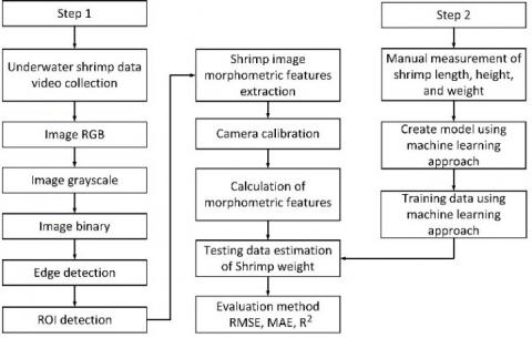
This research has two stages, the first stages of research carried out are (a) data retrieval of shrimp using underwater camera, (b) processing of shrimp video into Red Green Blue (RGB) images, (c) processing of RGB images into grayscale images, (d) processing of grayscale images into binary images using the Otsu algorithm, (e) edge detection of shrimp images (f) detecting the Region of Interest (ROI) of shrimp objects, (g) shrimp image morphometric features extraction, (h) camera calibration using Triangle Similarity (TS) and Correction Factor (CF), (i) calculating of morphometric features value.
The second stages of research carried out are (j) manual measurement of shrimp length, height and weight of the shrimp with a measuring tool, (k) create model using machine learning approach, (l) training data using machine learning approach. After stages one and two, the process is carried out (m) testing data estimation of underwater shrimp body weight, (n) evaluation method using Root Mean Square Error (RMSE), Mean Absolute Error (MAE), Coefficient of Determination (R2). A detailed stages of the research process is shown in Figure 1.
Image segmentation is the initial process of digital processing [28]. The digital image obtained is then preprocessed using the aforementioned procedure. It involves a series of steps, namely grayscale, binary image, and edge detection [29]. The contours of the shrimp are obtained from the image and are saved as separate files.
The first stage of image segmentation involves changing the color into a grayscale [30]. However, such images have a pixel value within the range of black and white. The black side is the weakest while the white has the strongest value [31]. The grey value corresponds with the brightness capacity [32]. The next step is to change the grayscale to a binary image [33]. This was realized using the thresholding method, which is the separation of objects between the foreground and background [34]. Furthermore, the pixel grouping is divided into the foreground and background grey levels [35]. The thresholding method is one of the main approaches in image segmentation [36].
The canny method, a type of edge detection process, was used to detect the shrimp image [37]. It is also used in image processing to determine the boundary of the object area [38-40]. In the present research, the canny method is used to detect the edges of shrimp. The adopted steps are image smoothing, and at each edge point, the maximum pixel is calculated in the gradient direction, these are found at the end point of the gradient [41].
The ROI is detected from the binary image obtained and used to provide certain restrictions on digital images [42]. This is carried out to ensure that the image processing procedure is only located in the area detected as shrimp. The minimum limit of shrimp objects or the image is cropped with a square ROI and saved with a different file name [43].
Figure 1. Stages of the research process
Table 1. Morphometric features
|
Feature |
Feature description |
Symbol |
|
Shrimp length |
Shrimp frame length |
TL |
|
Height |
Shrimp frame height |
H |
|
Carapace length |
The length of the shrimp carapace |
CL |
|
Carapace height |
Shrimp carapace height |
CH |
|
Sixth segment length |
The length of the sixth pleon segment of shrimp |
SSL |
|
Second segment height |
The height of the second shrimp pleon segment |
SSH |
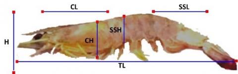
The extraction process is searching for unique feature information in the images, such as color, texture, and shape [44]. The morphometric features are characteristic of the shape of marine species. Luo et al. [27] stated that various characteristics, such as morphology, physiology, and behavior, are used to identify these species. However, this study recommended the extraction of shape features [20]. The morphometric features used are Total Length (TL), Height (H), Carapace Length (CL), Carapace Height (CH), Sixth Segment Length (SSL), Second Segment Height (SSH). In detail the morphometric features are shown in Table 1 and Figure 2 [27].
Figure 2. The morphometric features of the shrimp image
Each morphometric feature is taken from two coordinate points in the image. This process is used to calculate the length of the morphometric features of the shrimp. The length between 2 points is calculated using the Euclidian distance. The coordinates of 2 points are symbolized by (ax, ay) and (bx, by). Euclidian distance is calculated using formula 1.
$d(a, b)=\sqrt{(b x-a x)^2+(b y-a y)^2}$ (1)
Camera calibration using TS and CF, this is because the distance between the shrimp and the camera determines the size of the captured image. The shrimp swim freely in water causes the distance from the camera and its position to vary [20]. TS using focal length to estimate length of shrimp in the pixel, focal length is the distance between the lens and the object on the camera. The estimated length of shrimp is calculated using formulas 2. Where P is the length of the shrimp captured by the camera in pixels, W is the original length of the shrimp measured in millimeters (mm), F is focal length measured in mm, D is the original distance between the shrimp and the camera measured in mm.
$P=(W * F) / D$ (2)
CF is used to analyze the image variables. It is also used to estimate the size of each image [45-47]. CF is a feature calculation method that uses the ratio of the image to determine the pixel and actual sizes [20, 48]. The Correction Factor depends on the ratio of the original shrimp length to the image caught on camera (millimeter/pixel). It is also used to calculate all the values of the image features. The correction factor and the value of the shrimp image features are obtained using formulas 3 and 4.
$c f=\frac{p_t}{p_m}$ (3)
$V_f=V_o x c f$ (4)
where, $c f$ is the correction factor, $p_t$ is the value of the original shrimp length measured using a measuring tool in millimeters $(\mathrm{mm})$, and $p_m$ is the value of the length of the shrimp in pixels. $V_f$ is the final value of the shrimp image feature, $V_o$ is the shrimp image feature with units of pixels.
Predictions were processed using machine learning, namely, Multiple Linear Regression (MLR), Support Vector Machine (SVM), Random Forest (RF), Decision Tree (DT), K-Nearest Neighbor (KNN), Back Propagation Neural Network (BPNN), and Principal Component Regression (PCR).
MLR is a statistical algorithm that aims to determine the predictive results of the y variable. Y is the prediction result of each X input [49, 50]. The general formula for the MLR algorithm is stated in formula 5. Where Y is the dependent or response variable, $x_1, x_2 \ldots, x_n$ is the independent variable, $b_1, b_2, \ldots, b_n$ is the regression coefficient, a is a constant, and e is the error value.
$Y=a+b_1 x_1+b_2 x_2+\cdots+b_n x_n+e$ (5)
SVM is a supervised learning method that can be used for regression and classification. SVM has several kernels, including the linear kernel, polynomial kernel, and Radial Basis Function (RBF) kernel [51]. RF is a machine learning algorithm, a collection of decision trees. RF can be used for the regression and classification of large data sets. RF works by constructing a decision tree to get the regression results [52]. DT is a machine learning algorithm that applies to make decision rules like a tree structure. DT is a supervised learning method that can be used for classification and regression [53].
KNN is an algorithm that classifies data based on similarity to other data. For the case of KNN regression, it provides the introduction of the nearest K in the neighbor regression [54]. BPNN is a supervised learning method, which uses an output error to change its weight value in backwards. BPNN is a model that imitates the workings of the human brain, consists of an input layer, a hidden layer and an output layer, to get good results, BPNN requires training with a long time and large data [55]. PCR is predictive modeling approach which involves the use of Principal Component Analysis (PCA) and MLR, has been increasingly employed in various applications and industries [56]. It is also used to model predictions with several independent variables [57].
The accurate value is obtained using the RMSE, MAE, and R2. The most accurate value was predicted, with RMSE and MAE being the least, while R2 was the highest [58]. RMSE, MAE, and R2 are obtained using Eqns. (6)-(8), respectively.
$R M S E=\sqrt{\frac{1}{N} \sum_{I=1}^N\left(Y_{d a}-Y_{d p}\right)^2}$ (6)
$M A E=\frac{1}{N} \sum_{i=1}^N\left|Y_{d a}-Y_{d p}\right|$ (7)
$R^2=\frac{\left(\sum_{i=1}^N\left(Y_{d a}-Y_{d p}\right)\left(Y_{d p}-Y_{d w}\right)\right)^2}{\sum_{i=1}^N\left(Y_{d a}-Y_{d p}\right)^2 \sum_{i=1}^N\left(Y_{d p}-Y_{d w}\right)^2}$ (8)
where, $Y_{d a}$ is the original value, $Y_{d p}$ is the predictive value, $Y_{d w}$ is the mean value of the prediction, and $\mathrm{n}$ is the available data.
MLR is a statistical method that models a linear relationship between the independent variable and the dependent variable, MLR is evaluated using the lowest RMSE and MAE and the highest R2 [59]. PCA is a method for reducing data dimensions in images, and the main objective of the PCA method is to reduce dimensions so that image data is easier to process [60]. In this study PCA was used with MLR as a comparison algorithm called PCR. The highest the value of R2 indicates that the higher the relationship between the dependent and independent variables [61]. MLR is used for predictions using two or more variables, and a combination of variables is used as a regression equation [62].
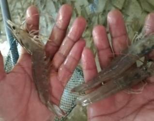
In this study, the data used is the image of shrimps underwater. The data collection was carried out in aquaculture ponds. The camera underwater used had a specification of 48 megapixels and lens focal length 26 mm. Lighting involves the use of two lamps above and inside the pool, a detailed scenario is shown in Figure 3 (a).
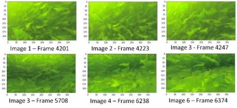
The data taken is video data of Mp4 type, then extracted into image frames, videos with a duration of 5 minutes produce 6,400 image frames. Extraction of videos into images using Python software with the OpenCV library. The function used to read the video file is cv2.videocapture(), and the function used to extract the video into an image is cam.read(). The images used in this study are 6 images, namely file frame 4201, frame 4223, frame 4247, frame 5708, frame 6238, and frame 6374 as shown in Figure 3 (b).
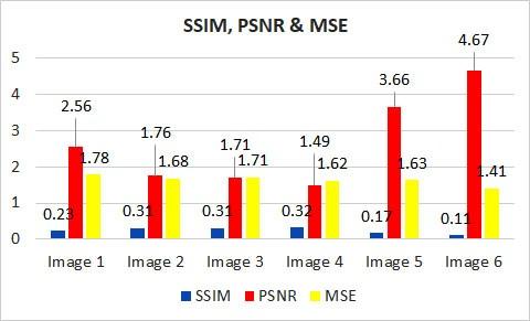
The experiment started with data preprocessing by converting RGB images into grayscale and binary images with a threshold value of 0.01 respectively. The conversion to a binary image was carried out using the Otsu algorithm. The results of the binary image process are evaluated using the Structural Similarity Index (SSIM). SSIM results are shown in the Figure 4.
(a) Data collection
(b) Underwater shrimp data
Figure 3. Shrimp image data collection
Figure 4. Value of SSIM, PSNR & MSE
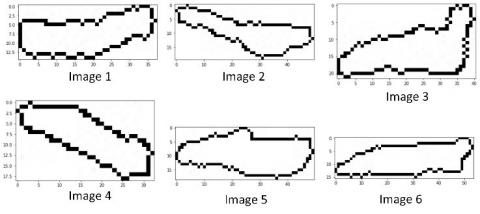
The edge detection process was carried out using a canny edge algorithm. This process is used to detect the edges of the underwater shrimp image. The canny is evaluated using Peak Signal Noise Ratio (PSNR) and Mean Square Error (MSE). A good edge detection result is an image that has the highest PSNR and the lowest MSE value. From the experimental results, the highest PSNR value is 4.67 and the lowest MSE is 1.41 on the image 6, as shown in Figure 4.
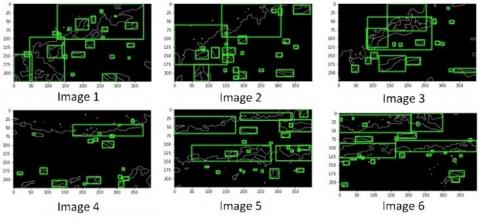
Regions of Interest (ROI) detection were used to detect the image's shape from several areas. The ROI detection results are shown in the Figure 5 (a). Amount of ROI detected image 1 = 23, image 2 = 23, image 3 = 17, image 4 = 17, image 5 = 24, image 6 = 25. From the detected ROI results, shrimp-shaped region was selected, then the invert image process is carried out, selected ROI image 1 = ROI 11, image 2 = ROI 19, image 3 = ROI 9, image 4 = ROI 10, image 5 = ROI 6, image 6 = ROI 14, as shown in Figure 5 (b).
(a) ROI detection
(b) Selected of shrimp shaped region
Figure 5. ROI detection and selected shrimp shaped region
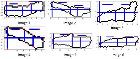
Figure 6. Result of image analysis for morphometric feature
Table 2. Morphometric features of six shrimp samples
|
TL |
H |
CL |
CH |
SSL |
SSH |
|
|
Image 1 |
38 |
15 |
10 |
9 |
7 |
8 |
|
Image 2 |
50 |
20 |
10 |
10 |
10 |
9 |
|
Image 3 |
41 |
22 |
8 |
9 |
7 |
9 |
|
Image 4 |
32 |
19 |
8 |
9 |
7 |
9 |
|
Image 5 |
50 |
19 |
10 |
13 |
10 |
16 |
|
Image 6 |
54 |
16 |
10 |
10 |
10 |
11 |
After obtaining the preprocessed data, it proceeded with the morphometric feature extraction process. A result of the image analysis for morphometric features is shown in Figure 6, the distance between 2 points is calculated using the formula 1. There are morphometric features for six shrimp samples with a detailed value in pixel shown in Table 2.
Camera calibration uses the focal length value of the camera lens, which is 26 mm The TS calculation uses the value of 1 shrimp which is measured manually, the distance between the shrimp and the camera with manual measurement is 51 mm, and the length of the shrimp measured manual is 106.6 mm. The cf value is calculated using formula 3, the result is 1.96 mm/pixel, this value is used to calculate the $V_f$ value of all morphometric features. The detailed $V_f$ calculation results are shown in Table 3.
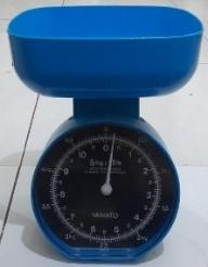
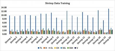
Create a machine learning model using 20 data of shrimp, morphometric characteristics and the body weight of shrimp was measured manually using a measuring tool, as shown in Figures 7 (a) and (b), value of 20 data training show in Figure 7 (c). Data of shrimp is used as training data, using machine learning algorithms.
Table 3. Morphometric features value result of TS-CF in centimeter
|
TL |
H |
CL |
CH |
SSL |
SSH |
|
|
Image 1 |
7.45 |
2.94 |
1.96 |
1.76 |
1.37 |
1.57 |
|
Image 2 |
9.80 |
3.92 |
1.96 |
1.96 |
1.96 |
1.76 |
|
Image 3 |
8.04 |
4.31 |
1.57 |
1.76 |
1.37 |
1.76 |
|
Image 4 |
6.27 |
3.72 |
1.57 |
1.76 |
1.37 |
1.76 |
|
Image 5 |
9.80 |
3.72 |
1.96 |
2.55 |
1.96 |
3.14 |
|
Image 6 |
10.59 |
3.14 |
1.96 |
1.96 |
1.96 |
2.16 |
(a) Shrimp measurement
(b) Measuring tool
(c) Shrimp data training
Figure 7. Manual measurement of shrimp and data training
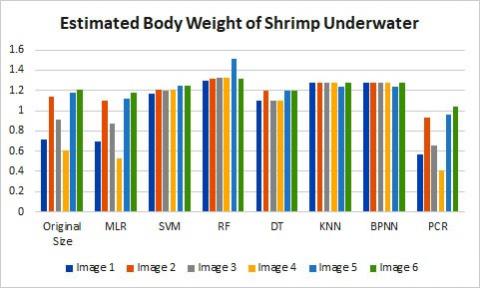
The weight of shrimp measured manually using a weighing tool showed the original weight of shrimp 1 = 0.71 g, shrimp 2 = 1.14 g, shrimp 3 = 0.91 g, shrimp 4 = 0.61 g, shrimp 5 = 1, 18 g, shrimp 6 = 1.21 g, with an average total weight = 0.96 g. Measuring of shrimp body weight estimation experiments using 6 data testing were carried out using machine learning methods, namely MLR, SVM, RF, DT, KNN, BPNN, and PCR.
From the original size, the MLR method produces an average shrimp weight decreased by 5.19%, the SVM method produces an average shrimp weight increase of 34.8%, the RF method produces an average shrimp weight increase of 49.63%, the DT method produces an average of shrimp weight increased 27.32%, KNN method produces an average of shrimp weight increased 42.32%, BPNN method produces an average of shrimp weight increased 42.32%, PCR method produces an average of shrimp weight decreased 21.85%. From these results, the standard deviation of the original size = 0.257, MLR = 0.266, SVM = 0.029, RF = 0.079, DT = 0.054, KNN = 0.016, BPNN = 0.016, PCR = 0.251. These results indicate the closeness of the standard deviation value of the original value and the 6 methods used, the smallest difference is the MLR method with a value of -0.009. The experimental results are shown in Figure 8.
Figure 8. Estimated body weight of shrimp underwater
Table 4. The results evaluation method
|
Method |
RMSE |
MAE |
R2 |
|
TS-CF-MLR |
0.05 |
0.04 |
0.96 |
|
TS-CF-SVM |
0.33 |
0.25 |
-0.99 |
|
TS-CF-RF |
0.44 |
0.39 |
-2.57 |
|
TS-CF-DT |
0.27 |
0.22 |
-0.36 |
|
TS-CF-KNN |
0.40 |
0.31 |
-1.84 |
|
TS-CF-BPNN |
0.39 |
0.31 |
-1.83 |
|
TS-CF-PCR |
0.65 |
0.65 |
-6.88 |
Table 4 shows the evaluation method uses RMSE, MAE, and R2. The results of the experiment show that the MLR algorithm produced the lowest RMSE and MAE error value is 0.05 and 0.04, and the highest R2 value is 0.96. SVM produced RMSE and MAE value is 0.33 and 0.25, and R2 value is < 0. The SVM was compared with MLR, and the RMSE and MAE values were increased by 28% and 2% respectively. RF produce RMSE and MAE value is 0.44 and 0.39, and the R2 value is < 0. The RF was compared with MLR, and the RMSE and MAE values were increased by 39% and 34% respectively. DT produce RMSE and MAE value is 0.27 and 0.22, and the R2 value is < 0. The DT was compared with MLR, and the RMSE and MAE values were increased by 22% and 17% respectively. KNN produce RMSE and MAE value is 0.4 and 0.31, and the R2 value is < 0. The KNN was compared with MLR, and the RMSE and MAE values were increased by 35% and 26% respectively. BPNN produce RMSE and MAE value is 0.39 and 0.31, and the R2 value is < 0. The BPNN was compared with MLR, and the RMSE and MAE values were increased by 34% and 26% respectively. PCR produce RMSE and MAE value is 0.19 and 0.19, and the R2 value is 0.29. The PCR was compared with MLR, and the RMSE and MAE values were increased by 14% and 14% respectively, while R2 was reduced by 24%.
MLR gets the best results because this method can identify how strong the influence of the independent variables is on the dependent variable. One variable, namely shrimp weight, was considered the explanatory variable, and the other was considered the dependent variable. Another thing that makes MLR the best method is that it is indeed used to predict values. This is in line with the function of the regression analysis which can be used for forecasting and prediction. This method is very suitable for to know the effect of two or more variables on the independent variable. Good estimation results are those that produce the lowest RMSE, MAE and the highest R2 values. The analysis results show that hybrid method TS-CF-MLR is the best result measuring estimation of the body weight shrimp underwater.
This study investigated the use of underwater image analysis and a machine learning approach for estimating underwater shrimp body weight using morphometric features with a non-invasive method. Among MLR, SVM, RF, DT, KNN, BPNN, and PCR algorithms which are combined with camera calibration using TS and CF, the MLR was able to produce the lowest RMSE, MAE, and the highest R2 as compared to all algorithms. This concludes that the TS-CF-MLR algorithm has higher accuracy estimated underwater shrimp body weight. Future research is the method developed in general can be applied to other animals, morphometric features can be used for all types of underwater animals, both fish and others. Monitoring systems using morphometric features, digital image analysis, and machine learning can be widely used in many artificial intelligence applications and the method used shows maximum accuracy results.
The authors are grateful to the Doctoral program of Information Systems, School of Postgraduate Studies, Diponegoro University for supporting this study.
|
d |
euclidian distance |
|
P |
length of the shrimp captured by the camera in pixels |
|
W |
original length of the shrimp measured in mm |
|
F |
focal length measured in mm |
|
D |
original distance between the shrimp and the camera measured in mm |
|
cf |
correction factor |
|
$V_o$ |
shrimp image feature with units of pixels |
|
$V_f$ |
final value of the shrimp image feature |
|
Y |
dependent variable MLR |
|
RMSE |
root mean square error |
|
MAE |
mean absolute error |
|
R2 |
coefficient of determination |
|
Pt |
value of the original shrimp length measured in mm |
|
Pm |
value of the length of the shrimp in pixels |
|
Greek symbols |
|
|
Σ |
sum of variables |
|
Subscripts |
|
|
x, y |
Image dimensions |
[1] Do, H.L., Ho, T.Q. (2022). Climate change adaptation strategies and shrimp aquaculture: Empirical evidence from the Mekong Delta of Vietnam. Ecological Economics, 196: 107411. https://doi.org/10.1016/j.ecolecon.2022.107411
[2] Ray, S., Mondal, P., Paul, A.K., Iqbal, S., Atique, U., Islam, M.S., Mahboob, S., Al-Ghanim, K.A., Al-Misnedg, F., Begum, S. (2021). Role of shrimp farming in socio-economic elevation and professional satisfaction in coastal communities. Aquaculture Reports, 20: 100708. https://doi.org/10.1016/j.aqrep.2021.100708
[3] Liu, Z. (2020). Soft-shell shrimp recognition based on an improved AlexNet for quality evaluations. J. Food Eng., 266: 109698. https://doi.org/10.1016/j.jfoodeng.2019.109698
[4] Adams, D., Donovan, J., Topple, C. (2021). Achieving sustainability in food manufacturing operations and their supply chains: Key insights from a systematic literature review. Sustainable Production and Consumption, 28: 1491-1499. https://doi.org/10.1016/j.spc.2021.08.019
[5] Anh, N.T.N., Shayo, F.A., Nevejan, N., Van Hoa, N. (2021). Effects of stocking densities and feeding rates on water quality, feed efficiency, and performance of white leg shrimp Litopenaeus vannamei in an integrated system with sea grape Caulerpa lentillifera. Journal of Applied Phycology, 33(5): 3331-3345. https://doi.org/10.1007/s10811-021-02501-4
[6] Chaikaew, P., Rugkarn, N., Pongpipatwattana, V., Kanokkantapong, V. (2019). Enhancing ecological-economic efficiency of intensive shrimp farm through in-out nutrient budget and feed conversion ratio. Sustainable Environment Research, 29(1): 1-11. https://doi.org/10.1186/s42834-019-0029-0
[7] Valenti, W.C., Barros, H.P., Moraes-Valenti, P., Bueno, G.W., Cavalli, R.O. (2021). Aquaculture in Brazil: past, present and future. Aquaculture Reports, 19: 100611. https://doi.org/10.1016/j.aqrep.2021.100611
[8] Liu, H., Liu, T., Gu, Y., Li, P., Zhai, F., Huang, H., He, S. (2021). A high-density fish school segmentation framework for biomass statistics in a deep-sea cage. Ecological Informatics, 64: 101367. https://doi.org/10.1016/j.ecoinf.2021.101367
[9] Liu, Z., Jia, X., Xu, X. (2019). Study of shrimp recognition methods using smart networks. Computers and Electronics in Agriculture, 165: 104926. https://doi.org/10.1016/j.compag.2019.104926
[10] Rashid, M., Nayan, A.A., Rahman, M., Simi, S.A., Saha, J., Kibria, M.G. (2022). IoT based smart water quality prediction for biofloc aquaculture. International Journal of Advanced Computer Science and Applications(IJACSA), 12(6): 56-62. https://doi.org/10.14569/IJACSA.2021.0120608
[11] Li, D., Hao, Y., Duan, Y. (2020). Nonintrusive methods for biomass estimation in aquaculture with emphasis on fish: A review. Reviews in Aquaculture, 12(3): 1390-1411. https://doi.org/10.1111/raq.12388
[12] Puig-Pons, V., Muñoz-Benavent, P., Espinosa, V., Andreu-García, G., Valiente-González, J.M., Estruch, V.D., Ordóñez, P., Pérez-Arjona, I., Atienza, V., Mèlich, B., de la Gándarad, F., Santaella, E. (2019). Automatic Bluefin Tuna (Thunnus thynnus) biomass estimation during transfers using acoustic and computer vision techniques. Aquacultural Engineering, 85: 22-31. https://doi.org/10.1016/j.aquaeng.2019.01.005
[13] Yeh, C.T., Chen, M.C. (2022). A combination of IoT and cloud application for automatic shrimp counting. Microsystem Technologies, 28(1): 187-194. https://doi.org/10.1007/s00542-019-04570-5
[14] Huang, J., Hung, C.C., Kuang, S.R., Chang, Y.N., Huang, K.Y., Tsai, C.R., Feng, K.L. (2018). The prototype of a smart underwater surveillance system for shrimp farming. In 2018 IEEE International Conference on Advanced Manufacturing (ICAM), pp. 177-180. https://doi.org/10.1109/AMCON.2018.8614976
[15] Yang, L., Yu, H., Cheng, Y., Mei, S., Duan, Y., Li, D., Chen, Y. (2021). A dual attention network based on efficientNet-B2 for short-term fish school feeding behavior analysis in aquaculture. Computers and Electronics in Agriculture, 187: 106316. https://doi.org/10.1016/j.compag.2021.106316
[16] Triantafyllou, A., Tsouros, D.C., Sarigiannidis, P., Bibi, S. (2019). An architecture model for smart farming. In 2019 15th International Conference on Distributed Computing in Sensor Systems (DCOSS), pp. 385-392. https://doi.org/10.1109/DCOSS.2019.00081
[17] Hao, M., Yu, H., Li, D. (2016). The measurement of fish size by machine vision - a review. In: Li, D., Li, Z. (eds) Computer and Computing Technologies in Agriculture IX. CCTA 2015. IFIP Advances in Information and Communication Technology, vol 479. Springer, Cham. https://doi.org/10.1007/978-3-319-48354-2_2
[18] Saberioon, M., Císař, P. (2018). Automated within tank fish mass estimation using infrared reflection system. Computers and Electronics in Agriculture, 150: 484-492. https://doi.org/10.1016/j.compag.2018.05.025
[19] Risholm, P., Mohammed, A., Kirkhus, T., Clausen, S., Vasilyev, L., Folkedal, O., Johnsen, Ø., Haugholt, K.H., Thielemann, J. (2022). Automatic length estimation of free-swimming fish using an underwater 3D range-gated camera. Aquacultural Engineering, 97: 102227. https://doi.org/10.1016/j.aquaeng.2022.102227
[20] Zhang, L., Wang, J., Duan, Q. (2020). Estimation for fish mass using image analysis and neural network. Computers and Electronics in Agriculture, 173: 105439. https://doi.org/10.1016/j.compag.2020.105439
[21] Yang, X., Zhang, S., Liu, J., Gao, Q., Dong, S., Zhou, C. (2021). Deep learning for smart fish farming: Applications, opportunities and challenges. Reviews in Aquaculture, 13(1): 66-90. https://doi.org/10.1111/raq.12464
[22] Chen, F., Xu, J., Wei, Y., Sun, J. (2019). Establishing an eyeball-weight relationship for Litopenaeus vannamei using machine vision technology. Aquacultural Engineering, 87: 102014. https://doi.org/10.1016/j.aquaeng.2019.102014
[23] Lin, H.Y., Lee, H.C., Ng, W.L., Pai, J.N., Chu, Y.N., Liou, C.H., Liao, K.C., Kuo, Y.F. (2019). Estimating shrimp body length using deep convolutional neural network. In 2019 ASABE Annual International Meeting (p. 1). American Society of Agricultural and Biological Engineers. https://doi.org/10.13031/aim.201900724
[24] Fernandes, A.F., Turra, E.M., de Alvarenga, É.R., Passafaro, T.L., Lopes, F.B., Alves, G.F., Singh, V., Rosa, G.J. (2020). Deep Learning image segmentation for extraction of fish body measurements and prediction of body weight and carcass traits in Nile tilapia. Computers and Electronics in Agriculture, 170: 105274. https://doi.org/10.1016/j.compag.2020.105274
[25] Thai, T.T.N., Nguyen, T.S., Pham, V.C. (2021). Computer vision based estimation of shrimp population density and size. In 2021 International symposium on electrical and electronics engineering (ISEE), pp. 145-148. https://doi.org/10.1109/ISEE51682.2021.9418638
[26] Poonnoy, P., Asavasanti, S. (2021). Implementation of coupled pattern recognition and regression artificial neural networks for mass estimation of headless‐shell‐on shrimp with random postures. Journal of Food Process Engineering, 44(8): e13747. https://doi.org/10.1111/jfpe.13747
[27] Luo, S., Li, Y., Gao, P., Wang, Y., Serikawa, S. (2022). Meta-seg: A survey of meta-learning for image segmentation. Pattern Recognition, 126: 108586. https://doi.org/10.1016/j.patcog.2022.108586
[28] Rehman, A., Ahmed Butt, M., Zaman, M. (2022). Liver lesion segmentation using deep learning models. Acadlore Transactions on AI and Machine Learning, 1(1): 61-67. https://doi.org/10.56578/ataiml010108
[29] Wu, C., Zhang, X. (2022). Total Bregman divergence-driven possibilistic fuzzy clustering with kernel metric and local information for grayscale image segmentation. Pattern Recognition, 128: 108686. https://doi.org/10.1016/j.patcog.2022.108686
[30] Hagara, M., Stojanović, R., Bagala, T., Kubinec, P., Ondráček, O. (2020). Grayscale image formats for edge detection and for its FPGA implementation. Microprocessors and Microsystems, 75: 103056. https://doi.org/10.1016/j.micpro.2020.103056
[31] He, H.J., Zheng, C., Sun, D.W. (2016). Image segmentation techniques. Computer Vision Technology for Food Quality Evaluation (Second Edition), 45-63. https://doi.org/10.1016/B978-0-12-802232-0.00002-5
[32] Mohan, V.M., Kanaka Durga, R., Devathi, S., Srujan Raju, K. (2016). Image processing representation using binary image; grayscale, color image, and histogram. In Proceedings of the Second International Conference on Computer and Communication Technologies, Springer, New Delhi, pp. 353-361. https://doi.org/10.1007/978-81-322-2526-3
[33] Du, S., Luo, K., Zhi, Y., Situ, H., Zhang, J. (2022). Binarization of grayscale quantum image denoted with novel enhanced quantum representations. Results in Physics, 39: 105710. https://doi.org/10.1016/j.rinp.2022.105710
[34] P. Smith, D.B. Reid, C. Environment, L. Palo, P. Alto, and P. L. Smith, A. (1979). Tlreshold selection method from gray-level histograms. IEEE Transactions on Systems, Man, and Cybernetics, pp. 62-66. https://doi.org/10.1109/TSMC.1979.4310076
[35] Senthilkumaran, N., Vaithegi, S. (2016). Image segmentation by using thresholding techniques for medical images. Computer Science & Engineering: An International Journal, 6(1): 1-13. https://doi.org/10.5121/cseij.2016.6101
[36] Halder, N., Roy, D., Roy, P., Roy, P. (2016). Qualitative comparison of OTSU thresholding with morphology based thresholding for vessels segmentation of retinal fundus images of human eye. IOSR Journal of VLSI and Signal Processing (IOSR-JVSP), 6(3): 41-48. https://doi.org/10.9790/4200-0603024148
[37] Huang, M., Liu, Y., Yang, Y. (2022). Edge detection of ore and rock on the surface of explosion pile based on improved Canny operator. Alexandria Engineering Journal, 61(12): 10769-10777. https://doi.org/10.1016/j.aej.2022.04.019
[38] Rasche, C. (2018). Rapid contour detection for image classification. IET Image Processing, 12(4): 532-538. https://doi.org/10.1049/iet-ipr.2017.1066
[39] Hu, X., Wang, Y. (2022). Monitoring coastline variations in the Pearl River Estuary from 1978 to 2018 by integrating Canny edge detection and Otsu methods using long time series Landsat dataset. CATENA, 209: 105840. https://doi.org/10.1016/j.catena.2021.105840
[40] Shanthi, S.A., Valarmathi, R. (2022). Edge detection on fuzzy near sets. Materials Today: Proceedings, 51: 2504-2511. https://doi.org/10.1016/j.matpr.2021.12.120
[41] Priyadharsini, R., Sharmila, T.S. (2019). Object detection in underwater acoustic images using edge based segmentation method. Procedia Computer Science, 165: 759-765. https://doi.org/10.1016/j.procs.2020.01.015
[42] Abdellatif, H., Taha, T.E., El-Shanawany, R., Zahran, O., Abd El-Samie, F.E. (2022). Efficient ROI-based compression of mammography images. Biomedical Signal Processing and Control, 77: 103721. https://doi.org/10.1016/j.bspc.2022.103721
[43] Xue, L., Hou, Y., Wang, S.W., Luo, C., Xia, Z,Y., Qin, G., Liu, S., Wang, Z.L., Gao, W.S., Yang, K. (2022). A dual-selective channel attention network for osteoporosis prediction in computed tomography images of lumbar spine. Acadlore Transactions on AI and Machine Learning. https://doi.org/10.56578/ataiml010105
[44] Jan, M.M., Zainal, N., Jamaludin, S. (2020). Region of interest-based image retrieval techniques: A review. IAES International Journal of Artificial Intelligence, 9(3): 520-528. https://doi.org/10.11591/ijai.v9.i3.pp520-528
[45] Fan, Q., Bi, Y., Xue, B., Zhang, M. (2022). Genetic programming for feature extraction and construction in image classification. Applied Soft Computing, 118: 108509. https://doi.org/10.1016/j.asoc.2022.108509
[46] Ap, D. (2014). Methodologies for studying finfish and shellfish biology. Central Marine Fisheries Research Institute. http://eprints.cmfri.org.in/id/eprint/10167, accessed on Sept. 16, 2022.
[47] Cárdenas, M., Filonzi, A., Delgadillo, R. (2021). Finite element and experimental validation of sample size correction factors for indentation on asphalt bitumens with cylindrical geometry. Construction and Building Materials, 274: 122055. https://doi.org/10.1016/j.conbuildmat.2020.122055
[48] Schrader, J., Shi, P., Royer, D.L., Peppe, D.J., Gallagher, R.V., Li, Y., Wang, R., Wright, I.J. (2021). Leaf size estimation based on leaf length, width and shape. Annals of Botany, 128(4): 395-406. https://doi.org/10.1093/aob/mcab078
[49] Ghodoosi, E.K., D'Alessandria, C., Li, Y., Bartel, A., Köhner, M., Höllriegl, V., Navab, N., Eiber, M., Li, W.B., Frey, E., Ziegler, S. (2018). The effect of attenuation map, scatter energy window width, and volume of interest on the calibration factor calculation in quantitative 177Lu SPECT imaging: Simulation and phantom study. Physica Medica, 56: 74-80. https://doi.org/10.1016/j.ejmp.2018.11.009
[50] Fan, B., Dai, Y., Zhang, Z., Wang, K. (2022). Differential SfM and image correction for a rolling shutter stereo rig. Image and Vision Computing, 124: 104492. https://doi.org/10.1016/j.imavis.2022.104492
[51] Singla, S.K., Garg, R.D., Dubey, O.P. (2020). Ensemble machine learning methods to estimate the sugarcane yield based on remote sensing information. Rev. d’Intelligence Artif, 34(6): 731-743. https://doi.org/10.18280/RIA.340607
[52] Singla, S. Y., Krecl, P., Targino, A.C. (2022). Fine-scale modeling of the urban heat island: A comparison of multiple linear regression and random forest approaches. Science of the Total Environment, 815: 152836. https://doi.org/10.1016/j.scitotenv.2021.152836
[53] Kamboj, U., Guha, P., Mishra, S. (2022). Comparison of PLSR, MLR, SVM regression methods for determination of crude protein and carbohydrate content in stored wheat using near Infrared spectroscopy. Materials Today: Proceedings, 48: 576-582. https://doi.org/10.1016/j.matpr.2021.04.540
[54] Mou, D., Wang, Z., Tan, X., Shi, S. (2022). A variational inequality approach with SVM optimization algorithm for identifying mineral lithology. Journal of Applied Geophysics, 204: 104747. https://doi.org/10.1016/j.jappgeo.2022.104747
[55] Gao, W., Zhou, Z.H. (2020). Towards convergence rate analysis of random forests for classification. Advances in Neural Information Processing Systems, 33: 9300-9311. https://doi.org/10.1016/j.artint.2022.103788
[56] Ghane, M., Ang, M.C., Nilashi, M., Sorooshian, S. (2022). Enhanced decision tree induction using evolutionary techniques for Parkinson's disease classification. Biocybernetics and Biomedical Engineering, 42(3): 902-920. https://doi.org/10.1016/j.bbe.2022.07.002
[57] Wang, Y., Pan, Z., Dong, J. (2022). A new two-layer nearest neighbor selection method for kNN classifier. Knowledge-Based Systems, 235: 107604. https://doi.org/10.1016/j.knosys.2021.107604
[58] De Luca, G., Gallo, M. (2020). The use of Artificial Neural Networks for extending road traffic monitoring data spatially: An application to the neighbourhoods of Benevento. Transportation Research Procedia, 45: 635-642. https://doi.org/10.1016/j.trpro.2020.03.047
[59] Meerasri, J., Sothornvit, R. (2022). Artificial neural networks (ANNs) and multiple linear regression (MLR) for prediction of moisture content for coated pineapple cubes. Case Studies in Thermal Engineering, 33: 101942. https://doi.org/10.1016/j.csite.2022.101942
[60] Swathi, K., Kodukula, S. (2022). Revue d ’ intelligence artificielle XGBoost classifier with hyperband optimization for cancer prediction based on geneselection by using machine learning techniques. Rev. d’Intelligence Artif, 36(5): 665-670. https://doi.org/10.18280/ria.360502
[61] Shams, S.R., Jahani, A., Kalantary, S., Moeinaddini, M. (2021). The evaluation on artificial neural networks ( ANN ) and multiple linear regressions ( MLR ) models for predicting SO2 concentration. Urban Climate, 37: 100837. https://doi.org/10.1016/j.uclim.2021.100837
[62] Akan, R., Keskin, S.N. (2019). The effect of data size of ANFIS and MLR models on prediction of unconfined compression strength of clayey soils. SN Applied Sciences, 1(8): 1-11. https://doi.org/10.1007/s42452-019-0883-8