Vera Mandailina* | Atin Nurhalimah | Saba Mehmood | Syaharuddin | Ibrahim
© 2022 IIETA. This article is published by IIETA and is licensed under the CC BY 4.0 license (http://creativecommons.org/licenses/by/4.0/).
OPEN ACCESS
Climate change is a global phenomenon that also causes small-scale effects. This study aims to determine future climate changes in the Mandalika International Circuit area using the artificial neural network of the MATLAB GUI-based backpropagation method. The simulation stage used daily rainfall intensity data collected in the Mandalika International Circuit area from 2012-2021 (365 data). A preliminary analysis concluded that the Mandalika International Circuit area is dominated by a very wet climate according to the Schmidt-Ferguson classification, which occurred in 2012, 2013, 2017, and 2021. This study used two architectural models with two and three hidden layers. The TRAINRP training function and the LOGSIG activation function were utilized at each hidden layer. Between the two architectures, the better architecture was selected, namely the 100-50-10-1 (three hidden layers) that resulted in an accuracy rate of 99.90% and an MSE of 0.0412376 achieved in the 258th iteration. These results indicate that the area has a very wet climate with the highest rain intensity in March and the lowest in January. The results of this study show that the backpropagation method can be used to help formulate an alternative policy on the measures for handling and mitigating extreme climate change in upcoming periods, especially during international events at the Mandalika International Circuit area.
neural network, backpropagation, climate change, Schmidt-Ferguson classification
Indonesia has recently hosted two international racing sports events, namely the WSBK (World Superbike) and MotoGP (Grand Prix Motorcycle) at Mandalika International Circuit. These events are prestigious motor racing sports events at the global level. Mandalika International Circuit is an arena used to hold international racing events located in the Mandalika Special Economic Zone (SEZ). In organizing such events, it is required to make efforts to anticipate climate conditions, especially the intensity of rainfall. According to Haliza [1], climate change can be defined as a change in the state of the climate. This change can be identified, for example by using statistical tests, by changes in the mean or variability of its properties that persist for a long time, usually for decades or longer.
Sari et al. [2] stated that forecasting is an activity to predict what will happen in the future. Siregar and Wanto [3] further elaborated that prediction is a presumption about the occurrence of an event in the future and forecasting is very helpful in planning and policy-making processes both in the government and non-government sectors. Predictive analysis is very important to conduct in a study so that the research becomes more precise and directed. Therefore, a good analysis using tested methods is needed so that the resulting accuracy can be truly accountable. Lee et al. [4] argued that rainfall prediction is essential to prevent floods, manage water resources, save lives and property, and secure economic activities.
One of the prediction methods widely used by researchers is artificial neural networks (ANN). Nogay et al. [5] stated that artificial neural network technology is one of the latest products of humanity's efforts in the research and imitation of nature. Artificial neural networks are programs designed to simulate the behavior of simple biological nervous systems. An artificial neural network is shaped by structuring a foreseen number of artificial neural cells in a certain architecture to process data. Nayak et al. [6] argued that artificial neural network algorithms have become an attractive inductive approach in rainfall prediction owing to their high nonlinearity, flexibility, and data-driven learning in building models without any prior knowledge about catchment behavior and flow processes. They are successfully used today in various aspects of science and engineering because of their ability to model both linear and non-linear systems without the need to make assumptions as are implicit in most traditional statistical approaches. The neural network has been used as a more effective model than simple linear regression. According to Abbot and Marohasy [7], the main advantage of neural networks lies in their ability to represent linear and non-linear relationships and the ability to learn these relationships directly from the data being modelled. Traditional linear models are inadequate for modeling data containing non-linear characteristics. This is emphasized by Chaturvedi [8] that an artificial neural network can be used for making predictions as it can examine and determine the historical data used for prediction. NN has a better accuracy than statistical and mathematical models. They work on the principle of biological neurons, which is a type of data-driven technique. The conjunction between meteorological parameters and rainfall can be analyzed using NN. Furthermore, Wahyuni et al. [9] stated that climate change in the world has caused a lot of impacts on changing rainfall patterns. This requires a method that can predict rainfall based on rainfall patterns that occur after climate change. Disasters can be anticipated with accurate information about how much rainfall will fall at a location in a certain period.
One of the important aspects of implementing backpropagation for forecasting rainfall is the change of seasons. According to Sharma and Nijhawan [10] and Govinda and Hiremath [11], backpropagation is the common method for training neural networks. This is a supervised learning method that requires a dataset of the desired output from many inputs, making up the training set and is most useful for the feed-forward network (networks that have no feedback or simply no connection in that loop). Hayat et al. [12] further described that the backpropagation algorithm architecture consists of three layers, namely the input layer, hidden layer, and output layer. At the input layer, there is no computational process, but at this layer, the X signal input occurs at the hidden layer. At the hidden and output layer, the computation process occurs for weight and bias, and the magnitude of the hidden output and output layer is also calculated based on certain activation functions. In this backpropagation algorithm, the binary sigmoid activation function was used because the expected output is between 0 and 1. At the input layer, the input was varied with Xn; while at the hidden layer there were weight (Vij) and bias (Voj), and Z as the hidden layer data. At the output layer, there are weight (Wij), bias (Woj), and Y as the output data.
The backpropagation method is a method that is quite well known and has been widely applied by previous researchers, including Jabjone [13] who applied artificial neural networks to predict rice yields in Thailand's Phimai District in 2002-2007. The results show that neural networks (8, 19, and 17) provided the lowest value of RMSE of 10.57 and MAPE of 2.3%. Naik and Pathan [14] also presented a modified backpropagation artificial neural network model for classifying and predicting Indian monsoon precipitation. The weather data were collected from the Meteorological Department with 80% of the total data were used for training purposes and 20% for validation purposes. The accuracy of the predictions achieved was between 80% and 90%, thus the neural networks were suitable for predicting precipitation. Lou et al. [15] also utilized backpropagation to determine the competitiveness evaluation of tourist attractions, with an accuracy rate of 97.3%.
According to Wu et al. [16], the artificial neural network model can recognize patterns of data through learning process and it has been applied to attain medical decision support. They utilized 15 data inputs with a single hidden layer architecture and obtained an accuracy rate of 85%. Furthermore, Wanto et al. [17] conducted a study to predict the Consumer Price Index (CPI) of the foodstuffs group using the artificial neural network backpropagation and fletcher reeves conjugate gradient. This study resulted in an accuracy rate of 75% and an MSE of 0.0142803691 using the backpropagation method with architecture of 12-15-1, the best architecture used. Lesnussa et al. [18] also utilized the artificial neural network of backpropagation to predict rainfall in the city of Ambon. This study utilized monthly rainfall data from 2011 to 2015 with a one-layer hidden 3-12-1 architecture. The results of training and testing data show that the accuracy rate of precipitation prediction obtained was 80% with an alpha of 0.7, an epoch of 10000, and an MSE value of 0.022.
According to Wahyuni et al. [9], based on their research a learning rate of 0.01, an architecture (4-5-3) of 4 inputs, 5 hidden layers, and 3 outputs with a maximum iteration of 1500 and error tolerance of 0.01 obtained the best results at the maximum iteration condition (1500) with an MSE value of 0.342. Setti and Wanto [19] analyzed the prediction of the highest number of internet users in the world using the backpropagation algorithm with a focus on data in 25 countries from 2013-2017. The accuracy result was 92% and the MSE was 0.0015 on the best network architecture of 3-50-1. In another study, Pamungkas et al. [20] applied the backpropagation to predict the production of Litopenaeus vannamei and Penaeus monodon shrimps in Indramayu Regency, which performed well during training. They recommended the trainGD function as a good training function with the lowest MAPE of 19.28%. Kouadri et al. [21] also evaluated the suitability of groundwater for human consumption and modelled water quality indices, temporally and spatially, using artificial neural networks. A total of 37 samples were harvested from eight different wells in the region throughout 2016 and the model recorded an MSE with an error rate of 9.3%. Pramita and Nusantara [22] applied backpropagation with architecture 144-10-5-1 for wind speed prediction reaching an accuracy rate of 99.9% with a learning rate of 0.7. In another study, Pramita and Nusantara [23] predicted an inflation rate using the backpropagation method and obtained an average yield of 0.213 with an MSE of 0.0053. They utilized a 120-10-5-1 architecture, trainrp as the training function and logsig as the activation function. The researchers utilized a combination of parameters to reduce the error rate of the architecture especially during training, testing, and prediction of data [24].
The results of these studies show that there have been many studies that apply the backpropagation neural network using two hidden layers. The input data used averaged 3-5 years, learning rate 0.7, and MSE value 0.0001-1.64. Therefore, so far, there is no research that uses backpropagation with three hidden layers and compares the accuracy results with two hidden layers. In addition, the learning rate that the researchers use is too large, where the role of learning rate accelerates the process of training and testing data but will affect the accuracy of the architecture. Therefore, one of the novelties in this research is to add a momentum parameter to the three hidden layer architecture to help reduce the resulting error. Furthermore, in this research we use data for the last 10 years, using a relatively small learning rate. We tested the architecture on a case study of rainfall data in the Mandalika International Circuit area. Hopefully, the prediction results can be used to determine rainfall trends in future and climate change in the region.
2.1 Data selection
This study used quantitative data to solve the research problems. The focus of the data used is the daily rainfall time series data in the Mandalika International Circuit area in Indonesia from 1 January 2012 to 31 December 2021 at 8.895oS and 116.306oE.
2.2 Research procedure
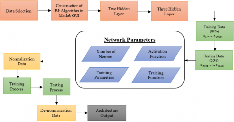
The accuracy parameter used in this forecasting was the Mean Square Error (MSE) and Root Mean Square Error (RMSE) assisted by MATLAB'S Graphical User Interface (GUI). Architectural design used to find the optimal NN configuration is also known as NN structural training, which consists of three NN layers, namely one input layer, one hidden layer, and one output layer. The number of neurons in the input layer and output layer depends on the problem itself [25, 26]. This is in line with Haviluddin and Alfred [27], who stated that the backpropagation network architecture generally consists of three layers, namely the input layer, the hidden layer, and the output layer. Similarly, the proper design of NN offers significant improvements to the learning system. Its components, such as nodes, weights, and layers are responsible for the development of various NN models. Single-layer perceptron (SLP) consists of input and output layers, making it the simplest form of an NN model [28]. The authors formulated and used simple and necessary research procedures for the research, as presented in Figure 1.
Figure 1. Flowchart of research
Based on Figure 1, after the data were obtained, the backpropagation algorithm was then determined using the MATLAB GUI. The artificial neural network model of the backpropagation method used to determine patterns was implemented to separate the data that will be used as training data (from 2012 to 2019 or 80%) and testing data (from 2020 to 2021 or 20%). Afterward, the prediction phase used data from 2012 to 2021 to predict rainfall data in 2022 (a 10 year-span). We use Z-score techniques to normalize and de-normalize the data (equation 1). The last stage of interplay and conclusion of the output results were obtained from the MATLAB R2013a GUI, with input results including graphs, epochs, prediction results, MSEs and RMSEs of each datum.
$Z=\frac{x_i-\bar{x}_i}{\sigma}$ (1)
2.3 Neural network backpropagation architecture
Backpropagation architecture consisting of input layer, hidden layer, and output layer was connected by activation and weight functions. Therefore, data prediction yk can be determined by formula:
$y_k=f\left(w_{0 k}+\sum_{j=1}^p w_{j k} \cdot f\left(v_{0 j}+\sum_{i=1}^n v_{i j} \cdot x_i\right)\right)$ (2)
Variables $x_1, x_2, \ldots, x_i, \ldots, x_n$ are an input layer determined by the amount of input data and only one layer, $y_1, y_2, \ldots, y_k$ are the output layer as well as one layer. In Eq. (2), $v_{11}, v_{1 j}, \ldots, v_{i j}$ are weight matrices that connect the input layer and the hidden layer, while $w_{11}, w_{1 k}, \ldots, w_{j k}$ are weight matrices that connect the hidden layer and the output layer.
Backpropagation architecture design was used to determine the best architecture with certain parameters through training and testing of previously shared data. In this study, the architectural parameters used were from the NN architecture of the backpropagation method using a learning rate of 0.1 and a momentum of 0.8. Previous research carried out by Mokhtar et al. [29] for data set 2 showed that learning rate of 0.1 and a momentum of 0.8 will generate the best result and the best network architecture achieved was 5-25-1. Syaharuddin et al. [30] in their research also showed that the learning rate value is recommended at intervals of 0.1-0.2 with a RE model value of 0.938 (very high), the momentum value at intervals of 0.7-0.9 with a RE model value of 0.925 (very high), and the number of neurons in the input layer that is smaller than the number of neurons in the hidden layer with a RE model value of 0.932 (very high). Complete information on the network architecture used is as follows
|
Setting Parameters: |
||
|
Max. Epoch |
: |
1000 |
|
Error (Goal) |
: |
0.001 |
|
Learning Rate (LR) |
: |
0.1 |
|
Momentum |
: |
0.8 |
|
Show Step |
: |
25 |
|
Activation Function |
: |
logsig (layer hidden) and purelin (layer output). |
|
Training Function |
: |
trainrp |
|
Amount of Neuron (2 layers hidden) |
||
|
Layer Input |
: |
10 years x 365 days (prediction data), 8 years x 365 days (training data), and 2 years x 365 days (testing data) |
|
Layer hidden-1 |
: |
100 |
|
Layer hidden-2 |
: |
50 |
|
Layer output |
: |
1 |
|
Amount of Neuron (3 layers hidden) |
||
|
Layer Input |
: |
10 years x 365 days (prediction data), 8 years x 365 days (training data), and 2 years x 365 days (testing data) |
|
Layer Hidden-1 |
: |
100 |
|
Layer Hidden-2 |
: |
50 |
|
Layer Hidden-3 |
: |
10 |
|
Layer Output |
: |
1 |
We set the parameters for the backpropagation architecture at the initial stage or before training and testing data. We use a binary sigmoid (logsig) activation function on each hidden layer according to Eq. (3).
$f(x)=\frac{1}{1+e^{-x}}$ (3)
3.1 Preliminary analysis results
The input of rainfall data for the Mandalika International Circuit area was obtained daily from 2012 to 2021, so 365 data were obtained for each year. The amount of rainfall (mm) calculated each month is displayed in Table 1.
Table 1. The input of rainfall data for the Mandalika International Circuit from 2012 to 2022
|
Month |
2012 |
2013 |
2014 |
2015 |
2016 |
2017 |
2018 |
2019 |
2020 |
2021 |
|
January |
158,42 |
139,12 |
140,54 |
125,64 |
15,18 |
203,89 |
173,24 |
56,6 |
37,54 |
290,62 |
|
February |
112,17 |
67,84 |
47,53 |
11,44 |
18,57 |
76,91 |
87,59 |
4,33 |
38,98 |
55,16 |
|
March |
110,34 |
28,81 |
27,62 |
10,61 |
4,71 |
68,53 |
32,53 |
18,67 |
15,98 |
79,2 |
|
April |
86,58 |
81,24 |
29,93 |
28,74 |
21,13 |
67,52 |
45,77 |
24,27 |
34,56 |
64,97 |
|
May |
178,7 |
142,23 |
88,85 |
23,97 |
94,87 |
116,33 |
114,26 |
69,01 |
49,93 |
132,35 |
|
June |
272,96 |
285,29 |
276,43 |
211,11 |
250,58 |
152,82 |
164,59 |
220 |
234,85 |
156,38 |
|
July |
296,17 |
288,77 |
281,64 |
161,29 |
183,68 |
264,85 |
270,96 |
231,66 |
211,46 |
206,95 |
|
August |
138,32 |
230,58 |
152,36 |
209,63 |
233,14 |
219,3 |
149,25 |
175,17 |
180,63 |
121,11 |
|
September |
287,1 |
261,98 |
202,85 |
226,52 |
265,41 |
202,57 |
218,53 |
148,01 |
228,49 |
232,83 |
|
October |
185,04 |
169,07 |
148,02 |
95,01 |
299,36 |
281,2 |
90,99 |
99,81 |
361,57 |
294,08 |
|
November |
187,25 |
273,03 |
146,92 |
125,23 |
137,15 |
196,93 |
148,86 |
172,01 |
190,86 |
257,18 |
|
December |
93,46 |
286,69 |
204,6 |
92,42 |
229,21 |
328,33 |
135,99 |
134,92 |
248,73 |
241,48 |
|
Q-value |
0 |
0,0909 |
0,3333 |
0,5 |
0,5 |
0 |
0,2 |
0,5 |
0,714 |
0,0909 |
|
Category |
Very wet |
Very wet |
Rather wet |
Rather wet |
Rather wet |
Very wet |
wet |
Rather wet |
Moderate |
Very wet |
Table 2. Data training and testing results
|
Hidden layer |
Stage |
Data |
Interval |
Amount of data |
Iteration |
MSE |
RMSE |
|
2 Hidden Layers (100-50-1) |
Training |
8 years (80%) |
2012-2019 |
8 x 365 |
376 |
0.0382 |
0.1954 |
|
Testing |
2 years (20% |
2020-2021 |
2 x 365 |
37 |
0.0526 |
0.2294 |
|
|
3 Hidden Layers (100-50-10-1) |
Training |
8 years (80%) |
2012-2019 |
8 x 365 |
133 |
0.0375 |
0.1936 |
|
Testing |
2 years (20% |
2020-2021 |
2 x 365 |
46 |
0.0502 |
0.2248 |
|
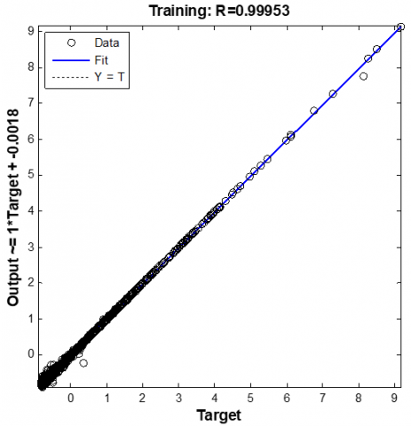
(a) Regression value H2-80% |
(b) Regression value H2-20% |
(c) Regression value H3-80% |
(d) Regression value H3-20% |
Figure 2. Plot regression of training and testing data
After calculating the amount of rainfall (mm) per month as seen in Table 1, it was discovered that in 2012, 2013, 2017, and 2021 the comparative value (Q) was 0 < Q < 0.143, so according to the Schmidt Ferguson Climate classification table, they are categorized as very wet months. Meanwhile, the years 2015, 2016, and 2019 obtained a ratio value of 0.600 < Q < 1,000 so they fall into the category of months with temperate climate. In 2014, the comparison value was 0.333 < Q < 0.600, making the months categorized as rather wet climate. However, the year 2020 had a very high comparison value (Q) of 0.714, making the monthsfall under the category of moderate.
Thus, from the results described above, it can be concluded that based on 10 years of rainfall data, the climate in Mandalika International Circuit area according to the Schmidt-Ferguson climate classification can mostly be categorized as very wet climate, which occurred in 2012, 2013, 2017, and 2021, or the peak of high rainfall. Meanwhile, the climate in 2014 was slightly wet; 2015, 2016, and 2019 were dominated by the medium climate; 2018 was mostly categorized as a wet climate; while 2020 was dominated by the extraordinarily dry climate or the peak of the long dry season occurring in the Mandalika International Circuit area.
3.2 Training, testing, and data prediction phase
Generally, there are two stages in the prediction process of NN backpropagation, namely the training and testing stages. According to Hayat et al. [31], the training stage uses data to produce results of backpropagation neural network training, while the testing stage implements the weight of NN from the training phase into the testing. In this study, the architectural pattern of the two hidden layers was 100-50-1 with an input layer of 365, a one hidden layer of 100, two hidden layers of 50 and an output layer of 1. Meanwhile, the architectural pattern for the three hidden layers was 100-50-10-1 with an input layer of 365, a one hidden layer of 100, two hidden layers of 50, three hidden layers of 10, and a layer output of 1. Data training and testing results are presented in Table 2.
Based on Table 2, the two hidden layers in the training stage obtained an MSE value of 0.0382 and RMSE value of 0.1954 achieved during the 376th epoch. Meanwhile, the testing stage obtained an MSE value of 0.0526 and RMSE value of 0.2294 achieved in the 37th epoch. Furthermore, the three hidden layers in the training stage obtained an MSE value of 0.0375 and RMSE value 0.1936 achieved in the 133rd epoch, and the testing stage obtained an MSE value of 0.0502 and RMSE value 0.2248 achieved in the 46th epoch. The training and testing results show that the architecture with three hidden layers performs well because the MSE and RMSE values are smaller when compared to the architecture with two hidden layers. Then, we strengthen this argument by looking at the pattern of data distribution according to the regression plot can be seen in Figure 2.
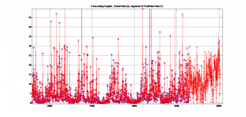
Based on Figure 2, we can see that the data distribution pattern using the architecture with three hidden layers is better than the architecture with two hidden layers. Then, the prediction of daily rainfall data in 2022 obtained results as presented in Figures 3 and Figure 4.
Figure 3. Results of daily rainfall prediction from actual data using two hidden layers
Figure 4. Results of daily rainfall prediction from actual data using three hidden layers
Based on Figure 3, the daily rainfall prediction using two hidden layers to process 10 years (10 x 365 data) obtained an MSE of 0.0417 and RMSE of 0.2047 achieved during the 172th. Meanwhile, the use of three hidden layers as shown in Figure 4 obtained an MSE of 0.0408 and RMSE of 0.2022 achieved during the 164th epoch. Thus, from these two architectural models, it was found that the three hidden layers (100-50-10-1) have predictive results derived from the actual data and can be used for forecasting calculations in future periods; or the MSE and RMSE value of three hidden layers is smaller than that of two hidden layers. This finding is supported by the research of Syaharuddin et al. [32] who argued that the determination of the best number of neurons on backpropagation using three layers with an architecture of 36-73-37-19-1 showed the highest level of accuracy at the time of precipitation data, obtaining an MSE of 0.0291 and an accuracy rate of 99.94% for data training and 99.99% for data testing.
Network performance can still be improved by increasing training data and replacing parameters that can affect performance such as error goals, epoch size, network architecture, and type of activation function. In the following, the authors present the 2022 rainfall forecasting results using two and three hidden layers, as seen in Table 3.
Table 3 shows the result of daily to monthly calculation for 2022 rainfall data in the Mandalika International Circuit area. Following the training stage, out of the two architectures, the best architecture resulted was the 100-50-10-1 (three hidden layers), where the very wet climate criteria according to the Schmidt-Ferguson classification would see the highest rainfall intensity in March with rainfall gains of 406.3721 mm and wet month descriptions, while the lowest rainfall intensity would happen in January with rainfall gains of 83.9642, making it classified as a humid month.
After finding out the climate change forecasting results, especially dynamic changes in the rainfall intensity in the Mandalika International Circuit area, the authors recommend the government or the organizers of WSBK (World Superbike) and MotoGP (Grand Prix Motorcycle) to hold these events in December or January. This aims to avoid high rainfall intensity such as those during previous events and to certainly minimize the occurrence of accidents due to slippery tracks during these events.
Table 3. Rainfall data prediction for 2022
|
Month |
Forecasting |
|||
|
Two Hidden Layers |
Three Hidden Layers |
|||
|
Rainfall (mm) |
Category |
Rainfall (mm) |
Category |
|
|
January |
520.8002 |
Wet month |
83.9642 |
Humid month |
|
February |
248.2224 |
Wet month |
264.5902 |
Wet month |
|
March |
527.2139 |
Wet month |
406.3721 |
Wet month |
|
April |
320.5872 |
Wet month |
290.0869 |
Wet month |
|
May |
297.8724 |
Wet month |
365.1046 |
Wet month |
|
June |
260.7365 |
Wet month |
245.302 |
Wet month |
|
July |
176.2403 |
Wet month |
257.8995 |
Wet month |
|
August |
199.3703 |
Wet month |
306.0636 |
Wet month |
|
September |
149.3004 |
Wet month |
282.586 |
Wet month |
|
October |
290.3435 |
Wet month |
299.5919 |
Wet month |
|
November |
366.5233 |
Wet month |
283.674 |
Wet month |
|
December |
584.0019 |
Wet month |
97.4145 |
Humid month |
|
Q-value |
0 |
|
0 |
|
|
Category |
Very Wet |
Very Wet |
||
Based on the Schmidt-Ferguson Criteria Climate Classification, the Mandalika International circuit area was dominated by the very wet climate in 2012, 2013, 2017, and 2021. Meanwhile, in 2014, the climate was moderately wet; 2015, 2016, and 2019 were dominated by the medium climate; 2018 was dominated by the wet climate; while 2020 was dominated by the extraordinary dry climate. The results obtained for two hidden layers in the training stage show an MSE of 0.0382 and RMSE of 0.1954, which was achieved in the 376th epoch, while in the testing stage, the authors obtained an MSE of 0.0526 and RMSE of 0.2294, achieved in the 37th epoch. On the other hand, using the three hidden layers in the training stage, the authors obtained an MSE of 0.0375 and RMSE of 0.1936 achieved during the 133rd epoch, while in the testing stage, the authors obtained an MSE of 0.0502 and RMSE of 0.2248 achieved in the 46th epoch. Furthermore, based on the implementation and testing carried out using the two architectural models, the best architecture obtained was the 100-50-10-1 (three hidden layers) with a "trainrp" training function and "logsig, logsig, logsig, purelin" activation function obtaining a MSE of 0.0408 and RMSE of 0.2022, which was achieved in the 164th epoch. This indicates that the climate of the Mandalika International circuit is a very wet climate with the highest rainfall intensity in March and the lowest rainfall intensity in January.
Therefore, the authors advise the government or organizers of WSBK (World Superbike) and MotoGP (Grand Prix Motorcycle) at the Mandalika International Circuit to avoid the high intensity rainfall such as those in the previous events. The authors recommend that these events be held in January or December to avoid slippery tracks and accidents during the races so that the activities may run optimally.
[1] Haliza, A.R. (2018). Climate change scenarios in Malaysia: Engaging the public. International Journal of Malay-Nusantara Studies, 1(2): 55-77.
[2] Sari, N.R., Mahmudy, W.F., Wibawa, A.P. (2016). Backpropagation on neural network method for inflation rate forecasting in Indonesia. International Journal of Advances in Soft Computing and Its Applications, 8(3): 69-87.
[3] Siregar, S.P., Wanto, A. (2017). Analysis of artificial neural network accuracy using backpropagation algorithm in predicting process (forecasting). IJISTECH (International Journal Of Information System & Technology), 1(1): 34. https://doi.org/10.30645/ijistech.v1i1.4
[4] Lee, J., Kim, C.G., Lee, J.E., Kim, N.W., Kim, H. (2018). Application of artificial neural networks to rainfall forecasting in the Geum River Basin, Korea. Water (Switzerland), 10(10): 1-14. https://doi.org/10.3390/w10101448
[5] Nogay, H.S., Akinci, T.C., Eidukeviciute, M. (2012). Application of artificial neural networks for short term wind speed forecasting in Mardin, Turkey. Journal of Energy in Southern Africa, 23(4): 2-7.
[6] Nayak, D.R., Mahapatra, A., Mishra, P. (2013). A survey on rainfall prediction using artificial neural network. International Journal of Computer Applications, 72(16): 32-40. https://doi.org/https://doi.org/10.5120/12580-9217
[7] Abbot, J., Marohasy, J. (2014). Input selection and optimisation for monthly rainfall forecasting in queensland, australia, using artificial neural networks. Atmospheric Research, 138: 166-178. https://doi.org/10.1016/j.atmosres.2013.11.002
[8] Chaturvedi, A. (2015). Rainfall prediction using back-propagation feed forward network. International Journal of Computer Applications, 119(4): 1-5. https://doi.org/10.5120/21052-3693
[9] Wahyuni, E.G., Fauzan, L.M.F., Abriyani, F., Muchlis, N.F., Ulfa, M. (2018). Rainfall prediction with backpropagation method. Journal of Physics: Conference Series, 983(1): 012059. https://doi.org/10.1088/1742-6596/983/1/012059
[10] Sharma, A., Nijhawan, G. (2015). Rainfall prediction using neural network. International Journal of Computer Science Trends and Technology, 3(3): 65-69. http://ijcstjournal.org/Vol3Issue3No1.html
[11] Govinda, K., Hiremath, S. (2014). Rainfall prediction using artificial neural network. International Journal of Applied Engineering Research, 9(23): 21243-21254. https://doi.org/10.29244/j.agromet.31.1.11-21
[12] Hayat, C., Soenandi, I.A., Limong, S., Kurnia, J. (2020). Modeling of prediction bandwidth density with backpropagation neural network (BPNN) methods. IOP Conference Series: Materials Science and Engineering, 852(1). https://doi.org/10.1088/1757-899X/852/1/012127
[13] Jabjone, S. (2013). Artificial neural networks for predicting the rice yield in Phimai district of Thailand. International Journal of Electrical Energy, 1(3): 177-181. https://doi.org/10.12720/ijoee.1.3.177-181
[14] Naik, A.R., Pathan, S. (2013). Indian monsoon rainfall classification and prediction using robust back propagation artificial neural network. International Journal of Emerging Technology and Advanced Engineering, 3(13): 99-101. https://doi.org/https://doi.org/10.1007/s00477-013-0695-0
[15] Lou B.N., Chen, N., Ma, L. (2020). Competitiveness evaluation of tourist attractions based on artificial neural network. Revue d'Intelligence Artificielle, 34(5): 623-630. https://doi.org/10.18280/ria.340513
[16] Wu, C.F., Wu, Y.J., Liang, P.C., Wu, C.H., Peng, S.F., Chiu, H.W. (2017). Disease-free survival assessment by artificial neural networks for hepatocellular carcinoma patients after radiofrequency ablation. Journal of the Formosan Medical Association, 116(10): 765-773. https://doi.org/10.1016/j.jfma.2016.12.006
[17] Wanto, A., Zarlis, M., Sawaluddin, Hartama, D. (2017). Analysis of artificial neural network backpropagation using conjugate gradient fletcher reeves in the predicting process. Journal of Physics: Conference Series, 930(1). https://doi.org/10.1088/1742-6596/930/1/012018
[18] Lesnussa, Y.A., Mustamu, C.G., Kondo Lembang, F., Talakua, M.W. (2018). Application of backpropagation neural networks in predicting rainfall data in Ambon city. International Journal of Artificial Intelligence Research, 2(2): 1-9. https://doi.org/10.29099/ijair.v2i2.59
[19] Setti, S., Wanto, A. (2019). Analysis of backpropagation algorithm in predicting the most number of internet users in the world. Jurnal Online Informatika, 3(2): 110. https://doi.org/10.15575/join.v3i2.205
[20] Pamungkas, A., Zulkarnain, R., Adiyana, K., Waryanto, Nugroho, H., Saragih, A.S. (2020). Application of Artificial Neural Networks to forecast Litopenaeus vannamei and Penaeus monodon harvests in Indramayu Regency, Indonesia. IOP Conference Series: Earth and Environmental Science, 521(1): 1-9. https://doi.org/10.1088/1755-1315/521/1/012018
[21] Kouadri, S., Kateb, S., Zegait, R. (2021). Spatial and temporal model for WQI prediction based on back-propagation neural network, application on EL MERK region (Algerian southeast). Journal of the Saudi Society of Agricultural Sciences, 20(5): 324-336. https://doi.org/10.1016/j.jssas.2021.03.004
[22] Pramita, D., Nusantara, T. (2020). Computational of distribution of wind speed as preliminary information for fishers: Case study in lombok sea. International Journal of Advanced Trends in Computer Science and Engineering, 9(3): 3584-3587. https://doi.org/10.30534/ijatcse/2020/165932020
[23] Pramita, D., Nusantara, T. (2021). Forecasting using back propagation with 2-layers hidden. Journal of Physics: Conference Series: 1845: 012030. https://doi.org/10.1088/1742-6596/1845/1/012030
[24] Challa, R.K., Rao, K.S. (2022). An effective optimization of time and cost estimation for prefabrication construction management using artificial neural networks. Revue d'Intelligence Artificielle, 36(1): 115-123. https://doi.org/10.18280/ria.360113
[25] Ojha, V.K., Dutta, P., Chaudhuri, A., Saha, H. (2015). Convergence analysis of backpropagation algorithm for designing an intelligent system for sensing manhole gases. In Hybrid Soft Computing Approaches: Research and Applications, 611: 215-236. https://doi.org/10.1007/978-81-322-2544-7_7
[26] Bai, Y., Li, Y., Wang, X., Xie, J., Li, C. (2016). Air pollutants concentrations forecasting using back propagation neural network based on wavelet decomposition with meteorological conditions. Atmospheric Pollution Research, 7(3): 557-566. https://doi.org/10.1016/j.apr.2016.01.004
[27] Alfred, R. (2016). A genetic-based backpropagation neural network for forecasting in time-series data. Proceedings - 2015 International Conference on Science in Information Technology: Big Data Spectrum for Future Information Economy, ICSITech 2015, pp. 158-163. https://doi.org/10.1109/ICSITech.2015.7407796
[28] Ojha, V.K., Abraham, A., Snášel, V. (2017). Metaheuristic design of feedforward neural networks: A review of two decades of research. Engineering Applications of Artificial Intelligence, 60: 97-116. https://doi.org/10.1016/j.engappai.2017.01.013
[29] Mokhtar, S.A., Wan Ishak, W.H., Norwawi, N.M. (2014). Modelling of reservoir water release decision using neural network and temporal pattern of reservoir water level. 2014 5th International Conference on Intelligent Systems, Modelling and Simulation, pp. 127-130. https://doi.org/10.1109/ISMS.2014.27
[30] Syaharuddin, S., Fatmawati, F., Suprajitno, H. (2022a). Best architecture recommendations of ANN backpropagation based on combination of learning rate, momentum, and number of hidden layers. JTAM (Jurnal Teori Dan Aplikasi Matematika), 6(3): 629-637. https://doi.org/https://doi.org/10.31764/jtam.v6i3.8524
[31] Hayat, C., Limong, S., Sagala, N. (2019). Architecture of back propagation neural network model for early detection of tendency to Type B personality disorders. Khazanah Informatika: Jurnal Ilmu Komputer Dan Informatika, 5(2): 115-123. https://doi.org/10.23917/khif.v5i2.7923
[32] Syaharuddin, S., Fatmawati, F., Suprajitno, H. (2022b). The formula study in determining the best number of neurons in neural network Backpropagation Architecture with Three Hidden Layers. Jurnal RESTI (Rekayasa Sistem Dan Teknologi Informasi), 6(3): 397-402. https://doi.org/https://doi.org/10.29207/resti.v6i3.4049