Khiat Salim* | Rahal Sidi Ahmed Hebri | Senaï Besma
© 2022 IIETA. This article is published by IIETA and is licensed under the CC BY 4.0 license (http://creativecommons.org/licenses/by/4.0/).
OPEN ACCESS
This study develops a condition classification system of compressor 103J and water pump systems which are key equipment in the ammonia production line, hence the monitoring of these two very important machines. In recent years, there are many good intelligent machine learning algorithms and XGboost is one of them. However, it contains many parameters and classification performance of the model will be greatly affected by the selection of parameters and their combination technique. In this paper, XGboost algorithm is combined with the genetic algorithm, called GA-XGboost, in order to find the best hyper parameters of classifiers which makes the classifier more efficient and ensures the proper functioning of compressor 103J and water pump systems. Experiments show that GA-XGboost algorithm has improved the accuracy of classification in the compressor 103J and the water pump dataset compared with other machine learning algorithms like Support Vector Machine (SVM), Random Forest (RF) and AdaBoost. Also experiments demonstrate the improvement of the GA-XGboost algorithm by the combination of different selection and crossover operators of the genetic algorithm.
data mining, genetic algorithm, machine learning, classification, random forest, XGboost algorithm
Predictive maintenance is the most effective way to ensure the sustainability of the commissioning of the production tool, thus increasing its production, its yield and the financial benefits which allow the company to remain in the competitive market of the production. Indeed, maintenance of equipment is a critical activity for any business involving machines and predictive maintenance; it has attracted much attention recently. It consists of planning maintenance based on the prediction about any equipment failure time. The prediction can be done by evaluating the data measurements from the equipment.
In the literature, there are two approaches to address the predictive maintenance problem. The first one is the classification approach in which it predicts the possibility of failure in next n-steps. The second one is the regression approach where it predicts the time left before the next failure, called Remaining Useful Life (RUL) [1, 2].
Recently, Machine learning has become leader on classification problems in the predictive maintenance. A classification model attempts to draw some conclusion from observed values. Given one or more inputs a classification model will try to predict the value of one or more outcomes. The model developed can be used to predict machine failure before it actually happens.
In recent works, many people have proposed different classification algorithm [3, 4]. For example, Praveenkumara et al. [5] performed the support vector machine (SVM) model for fault identification from the acquired vibration signals. They exposed the use of vibration signal for automated fault diagnosis of gearbox. Indeed, it showed better classification ability in identification of a several faults in the gearbox and it can be utilized for automated fault diagnosis. In the experimental studies, they used a good gears and face wear gears in order to compose vibration signals for good and faulty conditions of the gearbox. Each gear is experimented with two different speeds and loading conditions. In fact, the classification effectiveness of good and faulty gear with two different speeds and load conditions was carried out and the classification efficiency of four gears was quoted. On the other hand, [6, 7] used the well know classification algorithm random forest (RF).
Amihai et al. [6] used RF in order to predict the metrics derived from vibration data which represent the real-world industrial data. Indeed they presented an extensive case study based on vibration monitoring. They observed that the industrial assets can be predicted using machine learning performed to data from industrial site which is collected over 30 industrials pumps distributed at several sites during 2.5 years period. They performed experimental model with a classical persistence model. Before applying the random forest algorithm, they performed a pre-processing step where they prepared the data. They verified the obtaining results for some failures which showed that such failures could have been prevented with reliable predictions. Thus, their results are interesting for the applicability of machine learning in an industrial context.
Also Amihai et al. [7] used RF but for early detection of issues emerging in refrigeration and cold storage systems based on the followed features: Minimal sensor dependencies, high precision, and high generalizability of the learned model. They employed the trend decomposition and model learning using dynamic time warping and clustering for feature extraction and they learn the model using random forest-based algorithm that can indicate the presence or absence of an issue in any given refrigeration case at any given time. They performed some experiments on real data from 2265 refrigeration cases from different large supermarkets in order to validate their model. They obtained a precision of 89%, lead time of approximately seven days, and a recall of 46% when evaluated on unseen cases.
Additively Vasilić et al. [8] applied the Adaboost algorithm for classification terms of machine health. They proposed a method for state change detection in rotary machines. They repose on saved signals spectrogram analysis and characteristics appropriate for texture classification in digital images. The application of the Adaboost algorithm is proposed for thermal power plant fan mills whose impact plates are damaged during the coal grinding process. They tested their method on machine state classification in thermal power plant and demonstrated the robustness of the proposed model.
Other researchers combine the different machine learning algorithm [9] where they combined the random forests (RFs) method with extreme gradient boosting (XGboost) in order to establish the data-driven wind turbine fault detection framework. In the first stage, RFs is used to order the features by significance, which are either direct sensor signals or constructed variables from prior knowledge. Then in the second stage, XGboost algorithm trains the set of classifier for each particular fault based on the top-ranking features. Authors performed numerical simulations in order to verify the effectiveness of the proposed approach. In fact, they used the state-of-the-art wind turbine simulator FAST applied for three several types of wind turbines in both the below and above rated conditions. They observed that their approach is robust to different wind turbine patterns including offshore ones in several working conditions. They affirmed that the proposed ensemble classifier was able to protect against overfitting, and it achieved better wind turbine fault detection results than the support vector machine method when achieving with multidimensional data.
Finally Biswal and Sabareesh [10] developed a novel classification model based on the Artificial Neural Network (ANN) based on a bench-top test rig. It is indicate in order to mimic the operating condition of an actual wind turbine and utilize it for monitoring its condition so as to diagnose the incipient faults in its critical components. Authors performed the classification between healthy state features and faulty state features using ANN, yielding a classification efficiency of 92.6%.
In view of the above-mentioned works of predictive maintenance, many people have proposed different machine learning algorithm in recent years. One of them proposed the AdaBoost algorithm for classification step, other used either SVM algorithm for fault identification or Random Forest as a popular and robust machine learning algorithm for early detection of issues emerging in refrigeration and cold storage systems. Also other combined the random forests (RFs) method with extreme gradient boosting (XGBoost) in order to establish the data-driven wind turbine fault detection framework. And recently, other performed the ANN classifier in order to classify the vibration signature for the healthy condition as well as the faulty condition (gear tooth root crack and roller bearing inner race axial crack). Few works use the XGBoost algorithm in the classification phase in predictive maintenance while this algorithm is very powerful in the classification process. In recent years, XGboost algorithm [11] has been largely used by machine learning because of its fast processing speed and good model performance. And also it can be used in parallel with all CPU cores of the system to make better use of hardware. In this study, the XGboost algorithm is adopted for the classification process.
However, due to the too large number of XGboost hyper parameters that may affect the model performance, it is necessary to build a set of XGboost models by optimizing a set of hyper parameters that make the model perform better.
In light of the above-mentioned difficulties of hyper parameter optimization of the machine learning model, many researchers have proposed different enhancement optimization methods in recent years. For illustration, Xiang et al. [12] suggested particle optimization using particle swarm (PSO) inspired multi-elitist artificial bee colony algorithm. Maamri et al. [13] presented an ant colony optimization algorithm for parameter identification of Piezoelectric Resonator Chaotic System. Jodpimai et al. [14] proposed a set effort estimation using selection and genetic algorithms. Tarkhaneh et al. [15] proposed a new hybrid strategy for data clustering using cuckoo search (CSO) based on Mantegna levy distribution, PSO and k-means. Elsawy et al. [16] described a hybridized characteristic selection method in molecular classification utilizing CSO and GA, and Hussein and Jarndal [17] proposed GA, PSO and Artificial Bee Colony (ABC) Optimization Hybrid Model for GaN HEMT Parameter Extraction, and the like.
Since genetic algorithms give satisfactory results for parameter optimization search problems and give excellent results and solves the optimal solution, we opted for this algorithm. In this study, a learning and optimization model, extreme gradient boosting (XGboosting) and genetic algorithm are combined to improve the performance of compressor 103J and water pump fault classifier. These two ensemble models have already been employed in various classification applications, which have shown that XGboost with the genetic algorithm are effective and efficient classifier design algorithms.
This paper is organized as follows. Section 2 details the proposed approach. Section 3 describes the implementation details and the results. Finally, section 4 closes the paper with a discussion of observations as well as some ideas for future work.
2.1 XGBoost algorithm
The XGboost algorithm is better than the classical machine learning algorithm which only utilizes the first order derivative information, and it operates the second-order Taylor expansion on the loss function. The obtained optimal solution is more effective and at the same time lost. In order to decreases the variance of the model, makes the learned model easier, and saves the phenomenon of over-fitting, the regular term is added to the function.
XGboost algorithm is a scalable machine learning system for tree boosting that proposed by Chen and Guestrin [11]. In the competition Kaggle 2015, XGboost was the most popular model which 17 among 25 solutions used XGboost. The superior performance of XGboost in supervised machine learning is the reason why it is chosen to train the compressor 103J and water pump classifier in this study.
XGboost algorithm combines weak base learning models into a stronger learner iteratively. In deed at each iteration of gradient boosting, the residual will be utilized to correct the previous predictor that the indicated loss function can be optimized. The description of the parameters and Kernel used with XGboost is as follows:
Let $\mathrm{D}=\left\{\left(\mathrm{x}_{\mathrm{i}}, \mathrm{y}_{\mathrm{i}}\right)\right\}\left(|\mathrm{D}|=\mathrm{n}, \mathrm{x}_{\mathrm{i}} \in \mathbb{R}^{\mathrm{m}}, \mathrm{y}_{\mathrm{i}} \in \mathbb{R}^{\mathrm{n}}\right)$ represents a database with n examples and m features.
Eq. (1) represents the tree boosting model output $\hat{\mathrm{y}}_{\mathrm{i}}$ with K trees.
$\hat{y}_i=\sum_{k=1}^K f_k\left(x_i\right), f_k \in F$ (1)
where, $\left.\mathrm{F}=\{\mathrm{f}(\mathrm{x})) \omega_{\mathrm{q}}(\mathrm{x})\right\}\left(\mathrm{q}: \mathbb{R}^{\mathrm{m}} \rightarrow \mathrm{T}, \omega \in \mathbb{R}^{\mathrm{T}}\right)$ is the space of regression or classification trees. Each fk divides a tree into structure part q and leaf weights part ω. T denotes the number leaves in the tree.
The set of function fk in the tree model can be learned by minimizing the following objective function:
$\mathfrak{L}^{(t)}=\sum_{i=1}^n l\left(y_i, \hat{y}_i^{(t-1)}+f_t\left(X_i\right)\right)+\Omega\left(f_t\right)$ (2)
where the first term l in Eq. (2) is a training loss function which measures the distance between the prediction $\hat{\mathrm{y}}_{\mathrm{i}}$ and the object yi. And Ω represents the penalty term of the tree model complexity.
$\Omega\left(f_t\right)=\gamma T+\frac{1}{2} \lambda \sum_{j=1}^T \omega_j^2$ (3)
XGboost approximates Eq. (2) by utilizing the second order Taylor expansion and the final objective function at step t can be rewritten as:
$\mathfrak{L}^{(t)} \simeq \sum_{i=1}^n l\left(y_i, \hat{y}_i^{(t-1)}+g_i f_t\left(X_i\right)+\frac{1}{2} h_i f_t^2\left(X_i\right)\right)+\Omega\left(f_t\right)$ (4)
where gi and hi are first and second order gradient statistics on the loss function.
$g_i=\partial_{\hat{y}_i^{(t-1)}} l\left(y_i, \hat{y}_i^{(t-1)}\right), h_i=\partial^2 _{\hat{y}_i^{(t-1)}} l\left(y_i, \hat{y}_i^{(t-1)}\right)$ (5)
After removing the constant term and expandingΩ, Eq. (4) can be simplified as:
$\widetilde{\mathfrak{L}^{(t)}}=\sum_{i=1}^n\left[g_i f_t\left(X_i\right)+\frac{1}{2} h_i f_t^2\left(X_i\right)\right]+\gamma T+\frac{1}{2} \lambda \sum_{j=1}^T \omega_j^2=\sum_{j=1}^T\left[\left(\sum_{i \in l_j} g_i\right) \omega_j+\frac{1}{2}\left(\sum_{i \in l_j} h_i+\lambda\right) \omega_j^2\right]+\gamma T$ (6)
The solution weight $\omega_j^*$ of leaf j for a fixed tree structure q(x) can be obtained by applying the following equation:
$\omega_j^*=-\frac{\sum_{i \in l_j} g_i}{\sum_{i \in l_j} h_i+\lambda}$ (7)
After substituting $\omega_j^*$ into Eq. (6), there exists:
$\widetilde{\mathfrak{L}^{(t)^*}}=-\frac{1}{2} \sum_{j=1}^T \frac{\left(\sum_{i \in l_j} g_i\right)^2}{\sum_{i \in l_j} h_i+\lambda}+\gamma T$ (8)
where:
T: the number of leaf nodes,
And $\gamma$: the coefficient of this term,
Define Eq. (8) as a scoring function to evaluate the tree structure q(x) and find the optimal tree structures for classification. Nevertheless, it is impossible to search the whole possible tree structures q in practice.
2.2 Genetic algorithm
The Genetic Algorithm (GA) [18] is a processing model that simulates the evolutionary process of genetics and the natural evolution of Darwin’s biological evolution. It is usually used in the field of artificial intelligence to solve any optimization problem. It belongs to the evolutionary algorithm model. It takes all the individuals in a group as the object, and generates the next generation solution through operations such as: selection, crossover and mutation operators, which the initial population will be coded and performed until approximate the optimal solution. By utilizing the probability search technology, the information point iteration can be skipped to converge into the local optimal solution.
The selection operator consists in selecting the chromosomes in the population according to certain logic or rules in order to obtain a population that can be crossed. The crossover operator is utilized to identify the genetic rules of two crossing chromosomes, and then the operator identifies the gene sequence of the chromosomes of the children after the cross between two chromosomes. The mutation operator allows to directly changing, with a certain probability, the gene of a given chromosome.
The search flexibility is good, and the global optimal solution can be achieved rapidly. In addition, the algorithm directly uses the fitness feature value as the search information to discover the search direction and search rank, and solves the optimization problem that the objective function cannot be derived or the derivative does not exist. Among them, the five elements of parameter are:
2.3 GA-XGboost algorithm
While XGboost [19] has good results in all angles, there are still some problems, one of which is that it has many parameters, and several combinations of parameters get several result scores. In the field of algorithm parameter search, the genetic algorithm gives the excellent results and solves the optimal solution. However in this paper, the Genetic Algorithm is used to optimize the parameter search process of XGboost algorithm. XGboost settings help to control the model complexity, but can also add randomness to make the model training less sensitive to noise. XGboost has three main parameters sets which are Booster, General and Task, the main parts of each parameter sets are listed in Table 1.
Table 1. List of XGboost parameters
|
Type |
Parameter |
Default |
Description |
|
Booster |
Eta |
0,3 |
Shrinking the weight on each step |
|
Min_Child_Weight |
1 |
Defines the minimum sum of weights |
|
|
Max_depth |
6 |
Control over-fitting |
|
|
Gamma |
0 |
Specifies the minimum loss required to make a split |
|
|
Max_delta_step |
0 |
Help in logistic regression |
|
|
Subsample |
1 |
control the sample’s proportion |
|
|
Colsample_bytree |
1 |
Column’s fraction of randomly samples |
|
|
Colsample_bylevel |
1 |
Column for each split in each level |
|
|
Lambda |
1 |
L2 regularization term on weights |
|
|
Alpha |
1 |
L1 regularization term on weights |
|
|
Scale_pos_weight |
1 |
Helps in faster convergence |
|
|
General |
Booster |
Gbtree |
Select the model for each iteration |
|
Silent |
0 |
Output message switch |
|
|
Nthread |
Max |
Parallel processing and input the system core number. |
|
|
Task |
Objective |
Reg:linear |
Minimizing the loss function |
|
Eval_metric |
According to objective |
Validate data |
|
|
Seed |
0 |
Random seed |
In this paper, we select seven common parameters to be tuning: eta, Min_child_weight, max_depth, Gamma, Subsample, Nestimator and colsamplebytree.
Figure 1. GA-XGboost algorithm flow chart
Figure 1 describes the process of building the classification method: First, we divide the initial dataset into training and test dataset. After that, the hyper parameters of the XGboost classifier are adjusted with a genetic algorithm using the following four cases:
Case 01: Selection by rank and crossing at a single point.
Case 02: Selection by rank and uniform crossover.
Case 03: Selection by tournament and a single-point crossover.
Case 04: Selection by tournament and uniform crossover.
After we perform a mutation on new individuals; and finally, we use evaluation indicators to evaluate the model trained on the test dataset by using confusion matrix.
The pseudo code of GA-XGboost algorithm is reported below:
Algorithm: hyper parameter settings of the XGboost algorithm
Input: the training dataset D, the total number of iterations T and the size of the population G.
Results: The best set of hyper parameter values from XGboost.
t ← 0
Initialize the population randomly;
While t <T do
- T ← t + 1;
For g = 1 to G do
- Get the set of hyper parameter values from XGboost
- Divide D into 2 parts, the test dataset and the training dataset.
- Training the XGboost on the training set
- Get the value predicted using XGboost trained on the test set
- Calculate the values of true positive, true negative, false positive, false negative
- Calculate the value of the fitness function F1-Score for each individual
End for;
Choose individuals with the highest fitness value
Perform:
-Case 01: Selection by rank and crossover at a single point.
-Case 02: Selection by rank and a uniform crossover.
-Case 03: Selection by tournament and a single point crossover.
-Case 04: Selection by tournament and uniform crossover.
Perform a mutation on new individuals;
Generate the new population;
End while;
Returns the best set of hyper parameter values from XGboost;
The chromosomes contain 7 genes which correspond here to the hyper parameters to be refined; the genes have different codifications from each other and which correspond to the values that can potentially take hyper parameters. So we have the following genes detailed in Table 2:
• Eta: can vary from 0.01 to 1
• N_estimators: can vary from 10 to 2000
• Min_Child_Weight: can vary from 0.01 to 10.0
• Gamma: can vary from 0.01 to 10
• SubSample: can vary from 0.01 to 1.0
• ColsampleByTree: can vary from 0.01 to 1.0
• MaxDepth: can vary from 1 to 10.
Table 2. The hyper parameter modeling
|
Gene1 |
Gene2 |
Gene3 |
Gene4 |
Gene5 |
Gene6 |
Gene7 |
|
Eta |
N_estimators |
Max_depth |
Min_Child_Weight |
Gamma |
Subsample |
Colsample_bytree |
|
($\eta$) |
(N) |
$(\phi)$ |
$({\omega})$ |
$(\gamma)$ |
$(\alpha)$ |
$({\beta})$ |
2.3.1 Construction of the population
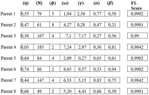
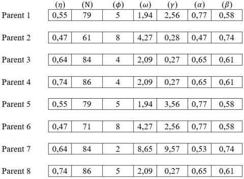
Figure 2 describes a population with 8 parents and 7 chromosomes where each one has 7 genes and each gene represents one hyper parameter of the XGboost algorithm.
Figure 2. Initial population
Initially, individual population which are the most able to reproduce are selected. In automatic learning, the capacity is measured by the capacity function (or quality or relevance or fitness). This study uses the parameters determined for the individuals to measure the F1-Score of XGboost. XGboost hyper parameters can vary and correspond to genes. After we will perform a selection, crossover and mutation operator to the initial population in four cases as described in the follow’s sections:
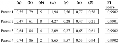
2.3.2 Selection by rank step
We will choose 4 parents who have a higher F1-Score value so we have the parents 1, parent 4, parent 5 and parent 6 with a F1-Score value of 0.9902 (see Figure 3).
Figure 3. Parents with the greatest F1-Score value
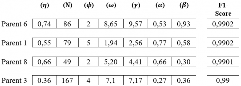
2.3.3 Selection by tournament step
In this step we will draw two individuals from our initial population at random and make them "fight". The one who has the highest fitness wins. So we will randomly select parents 4 and 6 and as the fitness value of parent 6 is higher than the fitness value of parent 4, we will select the parents 4 and 6. The fitness value of parent 6 is higher than that of parent 4 we will choose parent 6 for the crossing step.
Then we will randomly select parents 1 and 3 and as the fitness value of parent 1 is higher than that of parent 3, we will select parent 3 for the crossover step. The fitness value of parent 1 is higher than that of parent 3 so we will select parent 1 for the crossover step.
Then we will randomly select parents 8 and 4 and as the fitness value of parent 8 is higher than that of parent 4, we will select parent 1 for the crossing step. The fitness value of parent 8 is higher than that of parent 4 we will choose parent 8 for the crossing step.
At the end we will randomly select parents 7 and 3 and as the fitness value of parent 3 is higher than that of parent 4 we will choose parent 8 for the crossover step. The fitness value of parent 3 is higher than that of parent 7 we will choose parent 3 for the crossing step. So the parents that are selected for the crossover step are parents 6, 1, 8 and 3 for the crossover step (see Figure 4).
Figure 4. Parents selected after the tournament selection step
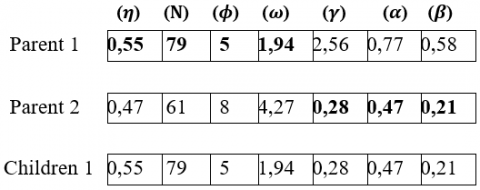
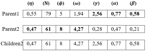
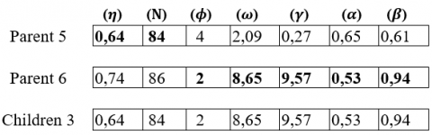
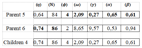
2.3.4 Crossover with single point step
After a crossover operator is performed with 1-point between parents 1 and 2 and also between parents 2 and 1 and also between parents 5 and 6 and between parents 6 and 5 as mentioned in Figure 5, Figure 6, Figure 7 and Figure 8.
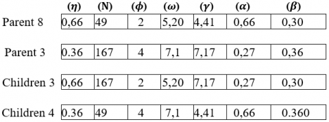
2.3.5 Uniform crossover step
In this step, a uniform crossover is made between parents 1 and 6 and between parents 8 and 3 with the mask 1011001. Figure 9 and Figure 10 show the results of the uniform crossover step.
Figure 5. Crossing at one point between parents 1 and 2
Figure 6. Crossing at one point between parents 2 and 1
Figure 7. Crossing at one point between parents 5 and 6
Figure 8. Crossing at one point between parents 6 and 5
Figure 9. Uniform crossover between parents 1 and 6
Figure 10. Uniform crossover between parents 8 and 3
2.3.6 Mutation step
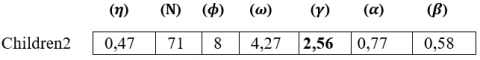
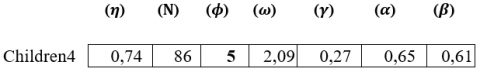
After the mutation simulation is done. In nature it's all about changes of the DNA sequence of a gene. In this study, this is a change in the value of a randomly drawn XGboost hyper parameter. So it is applied a mutation on Children 1, 2, 3 and 4 as mentioned in Figure 11, Figure 12, Figure 13 and Figure 14.
Figure 11. Mutation applied to gene 5 and children 1
Figure 12. Mutation applied to gene 2 and children 2
Figure 13. Mutation applied to gene 7 and children 3
Figure 14. Mutation applied to gene 3 and children 4
2.3.7 Building the novel population step
After the selection of the most suitable parents which have a higher F1-score value and after applying the crossover and mutation operator a new population or the generation 1 is constructed (see Figure 15).
Figure 15. The novel population
The genetic algorithm is an optimization technique based on chance. There is no guarantee that the new individuals will be better than the previous ones. So it must keep the old population at least to avoid serious results. The process is repeated until obtaining the optimal values of the hyper parameters of the XGboost algorithm.
This section investigates the representation of different experimentations performed intending to propose the optimal model toward the Predictive Maintenance for compressor 103J and water pump Systems.
3.1 Dataset source
Datasets used in this experiment are: The compressor 103J and the water pump (http://kaggle.com/nphantawee/pump-sensor-data) which are key equipment in the ammonia production line. The compressor dataset is a framework that collects data for monitoring of shaft vibration and axial displacement. The dataset is organized as an Excel file with 99969 data in the full dataset of which 42668 data classification labels are 0 (bad state) and the remaining 57300 data classification labels are 1 (good state). The dataset is a library dataset with 27 attributes described in Table 3.
Table 3. The 27 Compressor characteristics
|
Sensor |
Physical quantity |
Unit |
|
DEPAX1AD1 |
Axial displacement in the AX1AD position |
mm |
|
DEPAX3AD1 |
Axial displacement in the AX3AD position |
mm |
|
DEPAX3AD2 |
Axial displacement in the AX3AD position |
mm |
|
DEPAX6AD1 |
Axial displacement in the AX6AD position |
mm |
|
DEPAX6AD2 |
Axial displacement in the AX6AD position |
mm |
|
DEPAX8AD1 |
Axial displacement in the AX8AD position |
mm |
|
DEPAX8AD2 |
Axial displacement in the AX8AD position |
mm |
|
SP10SP01 |
Shaft speed |
rpm |
|
VIBVIB01HD |
Vibration in VIB 1HD position |
μm |
|
VIBVIB01VD |
Vibration in VIB1VD position |
μm |
|
VIBVIB02HD |
Vibration in VIB2HD position |
μm |
|
VIBVIB02VD |
Vibration in VIB2VD position |
μm |
|
VIBVIB03HD |
Vibration in VIB3HD position |
μm |
|
VIBVIB03VD |
Vibration in VIB3VD position |
μm |
|
VIBVIB04HD |
Vibration in VIB4HD position |
μm |
|
VIBVIB04VD |
Vibration in VIB4VD position |
μm |
|
VIBVIB05HD |
Vibration in VIB5HD position |
μm |
|
VIBVIB05VD |
Vibration in VIB5VD position |
μm |
|
VIBVIB06HD |
Vibration in VIB6HD position |
μm |
|
VIBVIB06VD |
Vibration in VIB6VD position |
μm |
|
VIBVIB07HD |
Vibration in VIB7HD position |
μm |
|
VIBVIB07VD |
Vibration in VIB7VD position |
μm |
|
VIBVIB08HD |
Vibration in VIB8HD position |
μm |
|
VIBVIB08VD |
Vibration in VIB8VD position |
μm |
The second dataset consist of a water pump. It is a library dataset with 51 characteristics which represent 51 sensors, namely precision sensor, temperature, oil density, vibration, speed, displacement. There are 220314 data in the full dataset which 14477 data classification labels are 0 (bad state) and the remaining 205836 data classification labels are 1 (Good state).
3.2 Experimental facility
Table 4 lists the hardware and software of the machine used for experimentations. The currently popular Tensorflow deep learning library is adopted for training.
3.3 Evaluation criteria for machine learning algorithms
In the classical method of classification learning, the classification precision (the ratio of the number of correctly classified samples to the total number of samples) is generally used as the evaluation index, but for the unbalanced dataset, the classification precision is used to evaluate the performance of the model. Therefore, in this study four evaluations criteria are used, such as Accuracy, Precision, Recall and F1-Value (F1-Score). These evaluation methods are based on the confusion matrix described in Table 5.
Table 4. Hardware and Software of computer
|
Item |
Content |
|
Google Colab -GPUs -CPUs -RAM Python Library
|
Public Google Colab - GPUs: K80 - 2xvCPU - 12GB Pandas Scikit-learn [20] Numpy Matplotlib Python 3.5 [21] |
Table 5. Confusion matrix of classification problems
|
Classification results |
Actual positives |
Actual negatives |
|
Positive results Negative results |
TP FN |
FP TN |
In the Table 5, TP (True Positives), TN (True Negatives), FN (False Negatives), and FP (False Positives) respectively indicate the positive and negative examples of the correct classification and the number of positive and negative examples of classification errors.
Accuracy:
Accuracy $=\frac{T P+F P}{T P+F N+T N+F P}$ (9)
Accuracy is used to measure the overall accuracy of the classification. The higher the accuracy, the better the classification effect.
Precision:
Precision $=\frac{T P}{T P+F P}$ (10)
Precision is used to reflect the proportion of positive cases that are correctly judged to be positive.
Recall:
Recall $=\frac{T P}{T P+F N}$ (11)
Recall is used to reflect the proportion of positive cases that are correctly judged to the total positive case.
F-Value:
$F-$ Value $=\frac{\left(1+\beta^2\right) \times \text { Precision } \times \text { Recall }}{\beta^2 \times \text { Precision }+\text { Recall }} \times 100$ (12)
F-Value is a classification evaluation index that comprehensively considers the Precision and Recall. When β=1, it is F1-Score.
3.4 Experimental results
In this paper, we will conduct two experiments on the two datasets. The first one consists of demonstrating the performance of XGboost with genetic algorithms compared to other machine learning algorithms. However the second one concerns the improvement of the performance of the XGboost algorithm with genetic algorithms by combining the different types of selection and crossover operators.
Figure 16. The experimental process
3.4.1 First experimentation: Experimental results GA-XGboost(case 01: selection by rank and single point crossover) with other algorithms
Figure 16 shows the experimental process indeed for pre-processing models, this section evaluates their performance attended by several classifiers including Support Vector Machine(SVM), Random Forest(RF), AdaBoost, XGboost and GA-XGboost (case 01) towards the two datasets (compressor 103J and water pump).
Preprocessing step.
The data cleaning step is important before the classification step. It consists of uniforming the data type and affecting the null data. The compressor 103J dataset contains different caracteristics data type for example : the displacement, vibration and speed are Object type and the state of compressor is Int type so all the caracteristics were converted into one data type which is float64.
Also the dataset compressor 103J contains 871887 null values. In this study the medium function is used in order to affect the null data. Table 6 exposes the dataset before and after Preprocessing.
Table 6. Comparative study of the compressor 103J dataset before and after Preprocessing
|
Dataset characteristics |
Before Preprocessing |
After Preprocessing |
|
Format |
Excel |
Excel |
|
Size |
99969, 27 |
99969, 24 |
|
Data type |
Object |
Float |
|
Values Null number |
871887 |
0 |
|
Class number labeled 0 |
42668 |
42668 |
|
Class number labeled 1 |
57300 |
57300 |
|
Name of the deleted characteristics |
No |
DEPAX7AD1 DEPAX7AD2 And Date and hour |
Table 7. Comparative study of the water pump dataset before and after Preprocessing
|
The dataset characteristics |
Before Preprocessing |
After Preprocessing |
|
Format |
Excel |
Excel |
|
Size |
220313,51 |
220313,50 |
|
Data type |
Float |
Float |
|
Values Null number |
220313 |
0 |
|
Class number labeled 0 |
14477 |
14477 |
|
Class number labeled 1 |
205836 |
205836 |
|
Name of the deleted characteristics |
No |
Sensor 15 |
In other hand, in the water pump dataset the sensor 15 contains 220313 null values which represent all sensor data values, so the characteristic sensor 15 will be deleted. Table 7 describes the water pump dataset before and after Preprocessing.
Classification step.
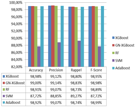
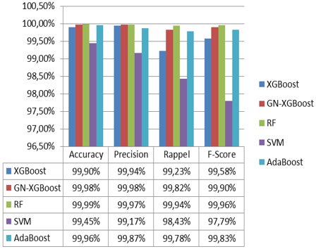
Figure 17 and Figure 18 show the experimental results of several classification algorithms applied both to the compressor 103J and the water pump dataset.
Figure 17 illustrates that the GA-XGboost gives the best Accuracy, precision, recall and F1-Score rate. The result with GA-XGboost is slightly better than the RF classification and the other classification algorithms for the four measures (accuracy, precision, recall and the F1-Score) except the AdaBoost algorithm where the F1-score value is slightly better that GA-XGboost.
From Figure 18, it can be seen that the best classification algorithm comes from RF algorithm instead of the others classification algorithms with the accuracy rate 99.99%, recall 99,94% and F1-score 99,96%.
Figure 17. Performance comparisons on the 103J compressor Dataset
Figure 18. Performance comparisons on the Water pump dataset
Followed by GA-XGboost algorithm with accuracy rate 99,98%. Therefore, the recall rate and F1-Score rate are slightly better with the RF algorithm than GA-XGboost and the other classifications algorithms. Therefor the precision rate is better with GA-XGboost algorithm than the other algorithm.
Discussions.
However, a comparative study is performed between the GA-XGboost algorithm and the most popular classification algorithms like XGboost, SVM, RF and AdaBoost.
In fact, Figure 17 shows that the four measures values of GA-XGboost are better than the others algorithms except the AdaBoost algorithm where the F1-score value is slightly better than GA-XGboost for the first dataset.
Nevertheless in the second dataset, the three measures (accuracy, recall and f1-score) values of RF are slightly better than the GA-XGboost algorithm except the precision value of GA-XGboost algorithm which is slightly greater than the RF.
This result is justified that the random forest algorithm is more suited to maintenance data like vibrations, movements, speed, pressure and temperature.... etc. Also the random forest algorithm is very adopted in the field of predictive maintenance based on the power of the decisions trees.
Since GA-XGboost gave satisfactory results in the first database, except for the F1-score measure, and in order to use it as a predictive maintenance model, we will improve this algorithm to give satisfactory results in all measures including F1-score. For this, we performed a series of combinations between the selection and crossover operators to improve the F1-score of the GA-XGboost which is the subject of the second experimentation.
3.4.2 Second experimentation: Experimental results GA-XGBoost with combining different kind of selection and crossover operators
This section exposes experimental results of the GA-XGboost algorithm by combining different selection and crossover operators in order to discover the best one that improve the performance of the GA-XGboost algorithm applied to the 103J compressor dataset. In this stage three cases are listed.
A. Selection by rank and uniform crossover (case 02)
This section represents the different parameters of the XGboost algorithm after using the genetic algorithm, using selection by rank operator and the uniform crossover operator with a population size of 100 in the 10 generations applied to the given 103J compressor set.
Table 8 represents the hyper parameters of the XGboost algorithm and also the value of F1-score in the ten generations, we notice that the best value of F1-score is 0.9908 and this value appeared in all generations. We can see that all generations have the same hyper parameters and also have the same value of F1-Score, so we can choose either the hyper parameters that appeared in all generations as the best hyper parameters of XGboost algorithm.
Table 8. XGBoost hyper parameters after using the selection by rank operator and the uniform crossover operator
|
Generation |
F1-Score |
($\eta$) |
(N) |
$(\phi)$ |
$({\omega})$ |
$(\gamma)$ |
$(\alpha)$ |
$({\beta})$ |
|
G0 |
0.9908 |
0.25 |
99 |
12 |
6.07 |
3.75 |
0.76 |
0.84 |
|
G1 |
0.9908 |
0.25 |
99 |
12 |
6.07 |
3.75 |
0.76 |
0.84 |
|
G2 |
0.9908 |
0.25 |
99 |
12 |
6.07 |
3.75 |
0.76 |
0.84 |
|
G3 |
0.9908 |
0.25 |
99 |
12 |
6.07 |
3.75 |
0.76 |
0.84 |
|
G4 |
0.9908 |
0.25 |
99 |
12 |
6.07 |
3.75 |
0.76 |
0.84 |
|
G5 |
0.9908 |
0.25 |
99 |
12 |
6.07 |
3.75 |
0.76 |
0.84 |
|
G6 |
0.9908 |
0.25 |
99 |
12 |
6.07 |
3.75 |
0.76 |
0.84 |
|
G7 |
0.9908 |
0.25 |
99 |
12 |
6.07 |
3.75 |
0.76 |
0.84 |
|
G8 |
0.9908 |
0.25 |
99 |
12 |
6.07 |
3.75 |
0.76 |
0.84 |
|
G9 |
0.9908 |
0.25 |
99 |
12 |
6.07 |
3.75 |
0.76 |
0.84 |
Table 9. The best XGBoost parameters after using the rank selection operator and the uniform crossover operator
|
Hyper parameter |
Before the optimization |
After the optimization |
|
LearningRate |
0.3 |
0.25 |
|
NEstimators |
100 |
99 |
|
MaxDepth |
6 |
12 |
|
MinChildWeight |
1 |
6.07 |
|
Gamma |
0 |
3.75 |
|
Subsample |
1 |
0.76 |
|
ColsampleByTree |
1 |
0.84 |
Table 10. XGBoost hyper parameters after using the tournament selection operator and the single point crossover operators
|
Generation |
F1-Score |
(η) |
(Ν) |
(ϕ) |
(ω) |
(γ) |
(α) |
(β) |
|
G 0 |
0.9894 |
0.34 |
223 |
11 |
3.22 |
6.37 |
0.11 |
0.28 |
|
G 1 |
0.9895 |
0.5 |
118 |
10 |
9.75 |
0.26 |
0.87 |
0.6 |
|
G 2 |
0.9895 |
0.18 |
235 |
11 |
3.92 |
7.22 |
0.87 |
0.87 |
|
G 3 |
0.9895 |
0.18 |
235 |
11 |
3.92 |
7.22 |
0.87 |
0.87 |
|
G 4 |
0.9895 |
0.54 |
230 |
14 |
1.54 |
0.01 |
0.87 |
0.87 |
|
G 5 |
0.9895 |
0.54 |
230 |
14 |
1.54 |
0.01 |
0.87 |
0.87 |
|
G 6 |
0.9895 |
0.52 |
118 |
13 |
4.7 |
2.67 |
0.96 |
0.81 |
|
G 7 |
0.9895 |
0.52 |
118 |
13 |
4.7 |
2.67 |
0.96 |
0.81 |
|
G 8 |
0.9895 |
0.29 |
115 |
2 |
9.66 |
0.36 |
1 |
0.7 |
|
G 9 |
0.9895 |
0.29 |
115 |
2 |
9.66 |
0.36 |
1 |
0.7 |
Table 11. The best XGBoost parameters after using the tournament selection and the single point crossover oprerators
|
Hyperparamètres |
Before the optimization |
After the optimization |
|
LearningRate |
0.3 |
0.29 |
|
NEstimators |
100 |
115 |
|
MaxDepth |
6 |
2 |
|
MinChildWeight |
1 |
9.66 |
|
Gamm |
0 |
0.36 |
|
Subsample |
1 |
1 |
|
ColsampleByTree |
1 |
0.7 |
Table 12. XGBoost hyper parameters after using the tournament selection operator and the uniform crossing operator
|
Generation |
F1-Scrore |
(η) |
(N) |
(ϕ) |
$({\omega})$ |
$(\gamma)$ |
$(\alpha)$ |
$({\beta})$ |
|
G0 |
0.9898 |
0.13 |
173 |
11 |
8.52 |
4.41 |
0.89 |
0.77 |
|
G1 |
0.9898 |
0.38 |
55 |
7 |
0.84 |
7 |
0.58 |
0.76 |
|
G2 |
0.9898 |
0.07 |
249 |
8 |
3.04 |
0.85 |
0.19 |
0.17 |
|
G3 |
0.9898 |
0.56 |
205 |
8 |
5.5 |
1.34 |
0.06 |
0.84 |
|
G4 |
0.9898 |
0.41 |
204 |
3 |
3.74 |
9.19 |
0.81 |
0.89 |
|
G5 |
0.9898 |
0.21 |
48 |
5 |
0.85 |
6.39 |
0.19 |
0.51 |
|
G6 |
0.9898 |
0.59 |
36 |
7 |
1.33 |
5.77 |
0.06 |
0.52 |
|
G7 |
0.9898 |
0.48 |
135 |
8 |
8.12 |
1.97 |
0.64 |
0.89 |
|
G8 |
0.9898 |
0.48 |
135 |
8 |
8.12 |
1.97 |
0.64 |
0.89 |
|
G9 |
0.9898 |
0.57 |
104 |
13 |
2.14 |
1.97 |
0.43 |
0.2 |
Table 13. The best XGBoost parameters after using the tournament selection and the uniform crossing operators
|
Hyperparamètres |
Before the optimization |
After the optimization |
|
LearningRate |
0.3 |
0.48 |
|
NEstimators |
100 |
135 |
|
MaxDepth |
6 |
8 |
|
MinChildWeight |
1 |
8.12 |
|
Gamm |
0 |
1.97 |
|
Subsample |
1 |
0.64 |
|
ColsampleByTree |
1 |
0.89 |
Table 14. Comparative study
|
|
Accuracy |
Precision |
Recall |
F1-Score |
|
Case 01: GA-XGboost : Single point crossover and selection by rank |
99% |
99.14% |
98.83% |
98.98% |
|
Case 02: GA-XGboost : uniform crossover and selection by rank |
99.04% |
99.18% |
98.87% |
99.02% |
|
Case 03: GA-XGboost : Single point crossover and tournament selection |
99% |
99.14% |
98.83% |
99.06% |
|
Case 04: GA-XGboost : uniform crossover and tournament selection |
99.08% |
99.21% |
98.90% |
99.05% |
After the optimization of XGboost by genetic algorithm with uniform crossing and selection by rank with a population of 100 parents and in 10 generations, the best combination of parameter is described in Table 9.
B. Tournament selection and single point crossover (Case 03)
This section represents the different parameters of the XGboost algorithm after using the genetic algorithm, using the tournament selection operator and the single point crossover operator with a population of size 100 in the 10 generations applied to the given set of compressor 103J.
Table 10 represents the hyper parameters of the XGboost algorithm and also the value of F1-score in the ten generations, we notice from Table 10 that the best value of F1-score is 0.9895 and this value appeared in all generations except the first generation which has a value of F1-score equal to 0.9894. We notice that each generation has different hyper parameters compared to the other generation except in the generation G4 and G5 we observe that these two generations have the same hyper parameters and also the generation G8 and G9 have the same hyper parameters but the hyper parameters which appeared in the generations G4 and G5 are different compared to the hyper parameters which appeared in the G 8 and G 9 and have the same value of F1-Score. So we can choose either the hyper parameters that appeared in G8 and G9 or in G4 and G6 as the best hyper parameters of the XGboost algorithm.
After the optimization of XGboost by genetic algorithm with a single point crossover and tournament selection with a population of 100 parents and in 10 generations, the best combination of parameters is presented in Table 11.
C. Selection tournament and Uniform crossover(Case 04)
This section represents the different parameters of the XGboost algorithm after using the genetic algorithm, using uniform crossover operator and the tournament selection operator with a population size of 100 in the 10 generations applied to the given 103J compressor dataset.
Table 12 represents the hyper parameters of the XGboost algorithm and also the value of F1-score in the ten generations, we notice that the best value of F1-score is 0.9898 and this value appeared in all generations. We show that each generation has different hyper parameters compared to the other generation except in the generation G7 and G8, we observe that these two generations have the same hyper parameters, as long as G7 and G8 have the same value of F1-score and also have the same hyper parameters so we can choose either the hyper parameters that appeared in G7 and G8 as the best hyper parameters of the XGboost algorithm.
After the optimization of XGboost by genetic algorithm with uniform crossover and tournament selection with a population of 100 parents and in 10 generations, the best combination of parameters is presented in Table 13.
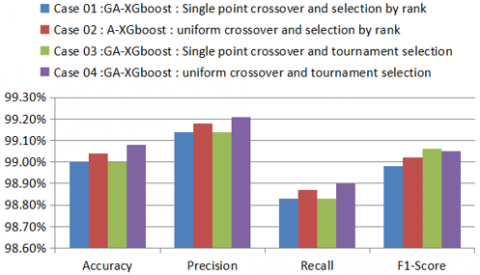
Comparison results.
In this section we will compare the results obtained from the optimization of the GA-XGboost algorithm using the four cases:
- Selection by tournament with crossover at a single point.
- Selection by tournament with uniform crossover.
- Selection by rank with uniform crossover.
- Selection by rank and single point crossover.
The results of these combinations are described in Table 14.
Figure 19. Comparative study
Figure 19 shows that the accuracy, precision and recall of GA-XGboost -uniform crossover and tournament selection exceed: the GA-XGboost -uniform crossover and rank selection, the GA-XGboost -single point crossover and rank selection, and the GA-XGboost - single point crossover and tournament selection. But the F1-score is slightly lower than GA-XGboost: Single point crossover and tournament selection.
Synthesis.
When performing the XGboost algorithm to the 103J compressor database, we obtained high accuracy where it is about 98.98% (Figure 17). We can say that this high value is due to three reasons, namely:
- The strength of the XGboost algorithm in classification because it depends on the pruned decision trees, and this means that the XGboost algorithm prunes the leaves of the trees, which makes the decision tree more accurate and powerful
- XGboost has several hyper parameters that allow us to control the implementation of the XGboost algorithm.
- The 103J compressor database which has been well cleaned and also well-organized.
As mentioned earlier, one of the reasons for the strength of the XGboost algorithm is that it has many hyper parameters, their adjustment makes the algorithm more efficient and powerful. To optimize these hyper parameters, we applied the genetic algorithm which is one of the most powerful algorithms in the field of optimization and finding optimal values. The basic principles of the genetic algorithm are the construction of a population, the most suitable individuals are selected, then a crossover is made between these individuals and finally a mutation is made in one of the genes of the individuals resulting from the crossover and we form a new population which is constituted by the most suitable individuals that were selected in the initial population and the children.
In case 01: Selection by rank and single point crossover, we noticed a slight improvement in all the performance criteria (accuracy, recall, precision and F1-score). Indeed according to Figure 17, the accuracy before the use of the genetic algorithm is equal to 98.98% and after the use of the genetic algorithm is equal to 99% with an improvement of 0.02%. Since we didn't have an important improvement, we tried in this work to change the crossover and selection operators because during the processing we observed that the parents that were selected in the stage of selection were always selected even after the stage of crossover and mutation.
So we can say that in spite of the crossover and mutation, the value of fitness of the children that were formed from the stage of crossover and mutation is lower than the value of fitness of the parents selected in the stage of selection. From Figure 19, we can say that selection by tournament and the single point crossover have the same value of accuracy with a slight improvement of 0.02% compared to the use of the XGboost algorithm without optimization. According to these results we can say that the best combination is the uniform crossover with tournament selection with accuracy of 99.08% and with a slight improvement of 0.1% compared to the XGboost algorithm without optimization and a slight improvement of 0.04% compared to the case 02 results.
In spite of the change of selection and the crossover method used in the case 01, we did not see a big difference between the results of this work and the results of case 01 and also we did not see a big improvement between the XGboost algorithm before and after the optimization because the results before optimization are already high and XGboost algorithm works well with small to medium size structured data and compressor 103J dataset does not exceed 100,000 lines.
On the other hand, Figure 19 shows the improvement F1-score=99.05% with GA-XGboost (case 04) compared with the F1-score=98.98 of GA-XGboost case 01. And also it is better than the Adaboost algorithm with the F1-score=98.99. So we can say the GA-XGboost case 04 is an efficient model for predictive maintenance for the compressor 103J. However RF is more efficient model for predictive maintenance for the Water Pump dataset.
This paper develops a classification system of the ammonia production chain for two keys machines state which are the compressor 103J and the water pump based to enhance the performance of predictive maintenance. The aim of this paper is to build classifier that can discover the damage stage of the two machines. Hence it proposes a XGBoost algorithm based on a combination of genetic algorithm global optimization parameters, called GA-XGboost algorithm. Due to its good performance, the practical application of the XGBoost model has involved various fields.
First a comparative study were conducted between GA-XGboost and other robust classifications algorithms such as SVM, Random Forest, AdaBoost and RF and shows that the proposed model has better classification performance using the compressor J103 dataset and RF has better classification performance using the water pump dataset.
In the second step, the improvement of the GA-XGboost algorithm is achieved by combining the different selection and crossover operators in four cases. Experiments showed that the best combination is the case 04: tournament selection and uniform crossover operators with 99.08% accuracy. Nevertheless, the execution time for processing the different genetic operations is significant. In the further research the implementation of the parallel version of GA-XGboost algorithm is necessary. Future research may also include the influence of recent optimization methods, such as Cuckoo search, on the performance of the method. Another idea would be to use other methods to solve similar problems with digital images for machine state classification.
The authors wish to thank the anonymous reviewers and the area editor for their constructive comments and helpful suggestions. Also, authors would like to express their very great appreciation to M. Bouriche Fares Master degree in Polytechnic National School of Oran (ENPO), for his valuable performing of the algorithm.
[1] Li, Z., He, Q. (2015). Prediction of railcar remaining useful life by multiple data source fusion. IEEE Transactions on Intelligent Transportation Systems, 16(4): 2226-2235. https://doi.org/10.1109/TITS.2015.2400424, 2015
[2] Mathew, V., Toby, T., Singh, V., Rao, B.M., Kumar, M.G. (2017). Prediction of Remaining Useful Lifetime (RUL) of turbofan engine using machine learning. In 2017 IEEE International Conference on Circuits and Systems (ICCS), 306-311. https://doi.org/10.1109/ICCS1.2017.8326010
[3] Khare, V., Kumari, S. (2022). Performance comparison of three classifiers for fetal health classification based on cardiotocographic data. Acadlore Transactions on AI and Machine Learning, 1(1): 52-60. https://doi.org/10.56578/ataiml010107
[4] Gullapelly, A., Banik, B.G. (2021). Classification of rigid and non-rigid objects using CNN. Revue d'Intelligence Artificielle, 35(4): 341-347. https://doi.org/10.18280/ria.350409
[5] Praveenkumar, T., Saimurugan, M., Krishnakumar, P., Ramachandran, K.I. (2014). Fault diagnosis of automobile gearbox based on machine learning techniques. Procedia Engineering, 97: 2092-2098. https://doi.org/10.1016/j.proeng.2014.12.452
[6] Amihai, I., Gitzel, R., Kotriwala, A.M., Pareschi, D., Subbiah, S., Sosale, G. (2018). An industrial case study using vibration data and machine learning to predict asset health. In 2018 IEEE 20th Conference on Business Informatics (CBI), 1: 178-185. https://doi.org/10.1109/CBI.2018.00028
[7] Amihai, I., Gitzel, R., Kotriwala, A.M., Pareschi, D., Subbiah, S., Sosale, G. (2018). An industrial case study using vibration data and machine learning to predict asset health. In 2018 IEEE 20th Conference on Business Informatics (CBI), 1: 178-185. https://doi.org/10.23919/ACC.2018.8431901
[8] Vasilić, P., Vujnović, S., Popović, N., Marjanović, A., Đurović, Ž. (2018). Adaboost algorithm in the frame of predictive maintenance tasks. In 2018 23rd International Scientific-Professional Conference on Information Technology (IT), 1-4. https://doi.org/10.1109/SPIT.2018.8350846
[9] Zhang, D., Qian, L., Mao, B., Huang, C., Huang, B., Si, Y. (2018). A data-driven design for fault detection of wind turbines using random forests and XGboost. IEEE Access, 6: 21020-21031. https://doi.org/10.1109/ACCESS.2018.2818678
[10] Biswal, S., Sabareesh, G.R. (2015). Design and development of a wind turbine test rig for condition monitoring studies. In 2015 International Conference on Industrial Instrumentation and Control (ICIC), 891-896. https://doi.org/10.1109/IIC.2015.7150869
[11] Chen, T., Guestrin, C. (2016). Proceedings of the 22nd acm sigkdd international conference on knowledge discovery and data mining. ACM, New York, USA, pp. 785-794. https://doi.org/10.1145/2939672.2939785
[12] Xiang, Y., Peng, Y., Zhong, Y., Chen, Z., Lu, X., Zhong, X. (2014). A particle swarm inspired multi-elitist artificial bee colony algorithm for real-parameter optimization. Computational Optimization and Applications, 57(2): 493-516. https://doi.org/10.1007/s10589-013-9591-2
[13] Maamri, F., Bououden, S., Boulkaibet, I. (2015). An ant colony optimization approach for parameter identification of piezoelectric resonator chaotic system. In 2015 16th International Conference on Sciences and Techniques of Automatic Control and Computer Engineering (STA), pp. 811-816. https://doi.org/10.1109/STA.2015.7505182
[14] Jodpimai, P., Sophatsathit, P., Lursinsap, C. (2018). Ensemble effort estimation using selection and genetic algorithms. International Journal of Computer Applications in Technology, 58(1): 17-28. https://doi.org/10.1504/IJCAT.2018.094061
[15] Tarkhaneh, O., Isazadeh, A., Khamnei, H.J. (2018). A new hybrid strategy for data clustering using cuckoo search based on Mantegna levy distribution, PSO and k-means. International Journal of Computer Applications in Technology, 58(2): 137-149. https://doi.org/10.1504/IJCAT.2018.094576
[16] Elsawy, A., Selim, M.M., Sobhy, M. (2019). A hybridised feature selection approach in molecular classification using CSO and GA. International Journal of Computer Applications in Technology, 59(2): 165-174. https://doi.org/10.1504/IJCAT.2019.098034
[17] Hussein, A.S., Jarndal, A.H. (2017). On hybrid model parameter extraction of GaN HEMTs based on GA, PSO, and ABC optimization. In 2017 International Conference on Electrical and Computing Technologies and Applications (ICECTA), pp. 1-5. https://doi.org/10.1109/ICECTA.2017.8252069
[18] Meng, X., Song, B. (2007). Fast genetic algorithms used for PID parameter optimization. In 2007 IEEE International Conference on Automation and Logistics, 2144-2148. https://doi.org/10.1109/ICAL.2007.4338930
[19] Swathi, K., Kodukula, S. (2022). XGBoost classifier with hyperband optimization for cancer prediction based on geneselection by using machine learning techniques. Revue d'Intelligence Artificielle, 36(5): 665-670. https://doi.org/10.18280/ria.360502
[20] Pedregosa, F., Varoquaux, G., Gramfort, A., Michel, V., Thirion, B., Grisel, O. (2011). Scikit-learn: Machine learning in Python. The Journal of Machine Learning Research, 12: 2825-2830.
[21] Paszke, A., Gross, S., Massa, F., Lerer, A., Bradbury, J., Chanan, G. (2019). Pytorch: An imperative style, high-performance deep learning library. Advances in neural information processing systems, 32: 8024-8035.