Prashanthi Peram* | Kumar Narayanan
© 2022 IIETA. This article is published by IIETA and is licensed under the CC BY 4.0 license (http://creativecommons.org/licenses/by/4.0/).
OPEN ACCESS
Infected by the novel coronavirus (COVID-19 – C-19) pandemic, worldwide energy generation and utilization have altered immensely. It remains unfamiliar in any case that traditional short-term load forecasting methodologies centered upon single-task, single-area, and standard signals could precisely catch the load pattern during the C-19 and must be cautiously analyzed. An effectual administration and finer planning by the power concerns remain of higher importance for precise electrical load forecasting. There presents a higher degree of unpredictability’s in the load time series (TS) that remains arduous in doing the precise short-term load forecast (SLF), medium-term load forecast (MLF), and long-term load forecast (LLF). For excerpting the local trends and capturing similar patterns of short and medium forecasting TS, we proffer Diffusion Convolutional Recurrent Neural Network (DCRNN), which attains finer execution and normalization by employing knowledge transition betwixt disparate forecasting jobs. This as well evens the portrayals if many layers remain stacked. The paradigms have been tested centered upon the actual life by performing comprehensive experimentations for authenticating their steadiness and applicability. The execution has been computed concerning squared error, Root Mean Square Error (RMSE), Mean Absolute Percentage Error (MAPE), and Mean Absolute Error (MAE). Consequently, the proffered DCRNN attains 0.0534 of MSE in the Chicago area, 0.1691 of MAPE in the Seattle area, and 0.0634 of MAE in the Seattle area.
load forecasting, COVID-19, neural network, pre-processing, data prediction, electricity
At the close of 2019, COVID-19 (C-19) appeared globally that possessed a critical effect on the international economy [1]. Businesses ceased, goods spoiled, manufacturing sequence stopped, and humans could not traverse the area. Due to C-19, businesses’ manufacturing and humans’ life was highly affected, thereby the electric load (EL) within the power system (PS) was as well vitally altered [2]. Being the economic advancement’s reference index, EL could cast the community’s financial condition. EL’s alterations during the C-19 pandemic (C-19P) became intricate. Electric appliances and lights are examples of electrical loads since they need electricity to function. A circuit's power consumption is another possible use of the phrase. As contrast to a power source, such as a battery or generator, which actually generates electricity Precise EL forecasting (ELF) could assure the community’s usual operation, efficiently lessen the operation charges of the PS, assure the power grid’s (PG) financial advantages, and enhance the social steadiness.
Normally, ELF’s intention remains in supervising the electric energy (EE) generation and dispensation scheduling [3]. Because of the PG’s strength and self-management capability, the EE variations resulting from local device fiascos and EL modifications would not create a crucial effect upon the PG. Hence, such little failings and turmoil could be disregarded in traditional forecasting (FC), and the FC outcomes will be fundamentally constant with the actuality [4]. Currently, numerous intelligent algorithms will be employed for FC EL. The deep learning (DL) algorithm allures great interest due to its robust learning capability and versatility [5].
Diverse neural networks (NNs) have been as well modeled to achieve the ELF’s distinct requirements in disparate settings [6]. Nevertheless, dissimilar to meteorological happenings, vacation, and the rest of the regular happenings, C-19P remains an irregular predicament. Furthermore, C-19’s effect upon EL consumes a lot of time. Relying upon C-19’s intensity and the counteractions embraced, the impact might persist for many months or indeed a year. The ELF paradigm’s training relies upon numerous sample data under standard circumstances. Also, the trained FC paradigm remains unsusceptible to an irregular crisis and possesses nil memory capability; thus, this remains evidently inappropriate for FC the EL of business during the C-19P. As C-19’s impact upon EL remains not a brief duration, this needs the FC paradigm to recall data sent via a lengthy duration.
The normal recurrent NN (RNN) [7] could not handle the data having lengthy-duration reliance and remains solely appropriate for the brief duration’s FC. Being a unique RNN type, NN could resolve this issue rightly [8]; hence, this remains very suitable for employing state-of-the-art RNN for FC EL of firms during the C-19P [9]. At standard conditions, the firms’ EL possesses cyclic variations because of the effect of air temperature (AT), time of day (ToD), season, public notion (PN), and government policy (GP) [10], and as well exhibits uniformity in the weekends and holidays. Besides, the EL’s historical data (HDt) of firms remains adequate [11]. Such features turn the firm’s ELF paradigm full-fledged. Nevertheless, correlated with the standard condition, this remains arduous in FC the firms’ EL because of the absence of experienced supervision whenever crises happen [12].
When there remains a paradigm, which could swiftly reply to happenings and provide great accurate FC outcomes, the PS’s capability in handling crises would be highly enhanced [13, 14]. Firms’ EL during the C-19P remains not merely influenced by standard features like AT, PN, GP, and ToD, yet as well influenced by clinical data [15, 16]. Moreover, unfinished data lead to sample data absence, which can be employed for paradigm training. This study’s inputs are:
This establishes the heterogeneous features concerned with electricity consumption (EC) and C-19’s condition into a load graph (LG) and constructs a graph portrayal learning paradigm for fitting the intricate mapping betwixt the current load status and the LF for the upcoming days.
To completely employ the concerned jobs’ knowledge, the present study applies multi-task learning (MTL) for building the Diffusion Convolutional RNN (DCRNN) by including criterion sharing layers for enhancing the normalization capability and FC precision.
The experimental results show the proposed model is better in handling load was evaluated using RMSE, MSE and MAPE.
This study is arranged as ensues: Segment 1 mentions the background of electricity demand and LF problems during C-19, Segment 2 highlights the associated studies for FC networks for EL, Segment 3 describes the proffered NN with FC layers, Segment 4 showcases the experimental assessment with graphs by error assessment, and, lastly, Segment 5 sums up this paper with a conclusion and prospective study.
Over the past few years, transfer learning and MTL are implemented in LF and attained extraordinarily splendid outcomes. Dissimilar to the general machine learning procedure, the DL procedure shows consideration for the appropriate time. As well, this remains essential in choosing data features for knowledge transition (KT).
The study [17] proffers a hybrid NN SLF paradigm centered upon a temporal convolutional network (TCN) and gated recurrent unit (GRU). Initially, the comparison betwixt meteorological features (MF) and load will be computed with the distance correlation coefficient, and the fixed-length sliding time window (STW) methodology will be employed for rebuilding the features. Then, TCN will be embraced for excerpting the hidden HDt and time association incorporating MF, electricity cost, and so on, and a finer-executing GRU will be employed for prediction.
The study [18] introduces a novel technique for SLF. This established methodology will be centered upon the amalgamation of convolutional NN (CNN) and long short-term memory (LSTM) networks. This methodology will be implemented in Bangladesh PS for giving short-term FC of EL.
The study [19] presents a hybrid NN, which incorporates CNN’s components (1D-CNN) and an LSTM network in new manners. Several individual 1D-CNNs will be employed for excerpting load, calendar, and weather features out of this proffered hybrid paradigm when LSTM will be employed in learning time patterns. The framework will be denoted as a CNN-LSTM network with multiple heads (MCNN-LSTM).
The study [20] suggests an SLF paradigm for regional dispensation networks incorporating the maximal data coefficient, factor assessment, gray wolf optimization, and normalized RNN (MIC-FA-GWO-GRNN). For screening and lessening the multiple-input features’ (IFs) size of the SLF paradigm, MIC will be initially employed for quantifying the non-linear correlation betwixt the load and IFs, and for removing the ineffectual features, and, later, FA will be employed for lessening the screened IFs’ size upon the presumption of sustaining the IFs’ chief data.
The study [21] contemplates a mid-term (MT) daily peak LF methodology employing recurrent artificial NN (RANN). An MT LF framework is implemented for surpassing such issues by input data (ID) substitution for special days and an RNN kind implementation.
The study [22] puts forth a direct paradigm for conditional probability density (PD) FC of residential loads centered upon a deep mixture network. Probabilistic residential LF (PRLF) could give overall data regarding prospective apprehensions in demand. An end-to-end composite paradigm consisting of CNNs and GRU will be modeled for PRLF. Next, the modeled deep paradigm will be fused with a mixture density network (MDN) for straightly predicting the PD functions (PDFs). Furthermore, multiple approaches, incorporating adversarial training, will be given to devise a novel loss function in the direct PRLF paradigm.
The study [23] employs a feature selection algorithm centered upon a random forest for giving a foundation for the IFs’ choosing of the LF paradigm. Subsequent to the choosing of IFs, a hybrid NN STLF algorithm centered upon multi-modal (MM) fusion will be proffered wherein the hybrid NN’s chief framework will be compiled of CNN and bidirectional GRU (CNN-BiGRU). The ID will be acquired by employing LST of disparate phases, and, later, the multiple CNN-BiGRU paradigms will be trained accordingly. The MMs’ FC outputs will be averaged for obtaining the last FC load value.
The study [24] puts forth 3 approaches – the nonlinear autoregressive exogenous paradigm (NARX) RNN, the Elman NN, and the autoregressive moving average (ARMA). The proffered approaches will be trained, authenticated, and tested by employing the historical record of hourly load data (LD) for the entire year 2018 that has been acquired out of the National Electrical Power Company (NEPCO).
The study [25] highlights the input attention mechanism (IAM) and hidden connection mechanism (HCM) for highly optimizing the RNN-related precision and effectiveness of LF paradigms. Particularly, the authors employ IAM for designating the significance weights upon input layers that possess finer execution in effectiveness and precision when compared with the conventional attention mechanisms. For additionally optimizing the paradigm’s effectiveness, HCM will be implemented for employing residual connection for optimizing the paradigm’s converging speed.
The study [26] introduces novel multiple parallel input and parallel output framework-related paradigms for FC EL power consumption. Focus has been made on the FC’s precision enhancement employing the novel framework constructed by the authors. These paradigms possess a capability in FC day-to-day load profiles having a lead time of 1 to 7 days.
Even though conventional CNN [27] execute nicely in text processing and data identification, they could just process data in Euclidean space. Thus, there remains enhancing attention in normalizing convolutions to the graph domain. DCRNN remains a favored methodology that learns node portrayals by forwarding and collecting messages betwixt adjacent nodes when sustaining the topological architecture. Nevertheless, a collection procedure with kth DCRNN layers employs k-order neighbors’ data. Consequently, DCRNN could over-smooth the portrayals while many layers have been stacked.
Overall in literature mentioned different existing models on load balancing has been illustrated with their advantages and limitations.
3.1 Problem formulation
In this study, the FC issue could be indicated as: Provided an array of LGs $\{G 1, G 2, G 3 \ldots G L\}, L=\frac{T L-T K}{n+1}$ and the real ensuing 24-hour load records as labels $\{y 1, y 2, \ldots y L\}$.The aim remains to learn a paradigm, which could create 24-hour FCs for hidden LG. We presume in having a dataset (DS) comprising the time series (TS) of electric power (EP) utilized by a building, averaged each quarter-hour $( QH )$, for a number $N$ of following days in the recent times. Particularly, the calculated values $y^{\sim} i(k)$ will be present, $k=1, \ldots, 96$, everyone portraying the mean EP utilized in the $k$ th $QH$ of the day $i , i=1, \ldots, N$.
Additionally, for similar days, we presume that weather measurements will be present as vector concatenation, $i(1), \ldots, u w, i(96), u w, i(k) \in R n W$. Weather vector elements in every time interval (TI) generally incorporate the external temperature, relative humidity, solar irradiation, and wind speed calculated by a weather station nearer to the regarded building. This issue could be classified as SLF. Employing the accessible DS encompassing N days, a one-day-ahead FC algorithm (FCA) needs to be inferred. Specifically, at each day’s start, the algorithm should predict the course of quarterly EC for that day alongside prediction error bounds. The algorithm would include the simulation, for a day, of a discrete-time autoregressive paradigm of order ny having appropriate predicted input indicators; we permit this paradigm to be established with the initial ny load measurements of the day. Hence, the inferred FCA would generate EC’s 96–ny predicted values at time phase ny of every day.
3.2 Proffered methodology
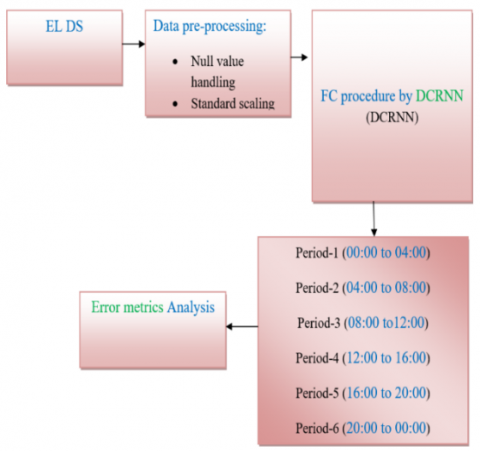
Figure 1. Flow chart of the ELF system for quarter-term LF using DCRNN
Figure 1 exhibits the block diagram of the ELF system for quarter-term LF. DCRNN will be employed to schedule the power systems ranging out of each 4 hours. Subsequent to implementing the data pre-processing, the powerful NN will be enhanced and established called DCRNN. The execution has been calculated upon the test set centered upon the standard execution error metrics like R-squared, MAPE, MSE, and RMSE. Lastly, the LF has been calculated and the execution has been analyzed concerning errors for real and predicted load demands.
3.3 Data pre-processing
A data point (DPt) di in this mechanism can be regarded as noise when its absolute value remains 4 times above the absolute medians of the 3 consecutive points prior to and subsequent to this DPt; i.e., $d_i$ remains the noise when its value fulfills the requirement: $d_i \geq 4 \times \max \left\{\left|m_a\right|,\left|m_b\right|\right\}$ in which $m_a=\operatorname{median}\left(d_{i-3}, d_{i-2}, d_{i-1}\right)$ and $m_b=\operatorname{median}\left(d_{i+3}, d_{i+2}, d_{i+1}\right)$. If the DPt remains recognized as noise, its value will be substituted by the 2 points’ mean value, which is present right away prior to and subsequent to this. TS $X$ can possess lacking value. A masking vector $m_t \in$ $\{0,1\}^D$ will be presented for indicating whatever variables remain lacking at time phase t and as well sustain the TI $\delta_t^d \in$ R for every variable d since its latest observance. To be extra precise, we have
$m_t^d=\left\{\begin{array}{cc}1, & \text { if } x_t^d \text { isobserved } \\ 0, & \text { otherwise }\end{array}\right.$
$\delta_t^d=\left\{\begin{array}{c}s_t-s_{t-1}+\delta_{t-1}^d m_{t-1}^d=0 \\ s_t-s_{t-1} t>1, m_{t-1}^d=1 \\ 0 . t=1\end{array}\right.$
Presume that, for every data 1 ≤ i ≤ I, we notice a form sequence {yi, wi, Xi} in which yi indicates a scalar result, wi indicates a scalar covariates' vector, and Xi indicates a data predictor (DP) computed above a lattice (a limited, connected gathering of vertices within a Cartesian coordinate system). The scalar regressionparadigm can be computed as,
$y i= w i T \Omega+ X i \beta+\mu i$
in which, $\Omega$ portrays a fixed-effects vector, $\beta$ portrays a regression coefficients' gathering described upon a similar lattice as the DPs, and $X i . \beta$ portrays the dot product of $X _i$ and $\beta$. The aim remains to analyze the coefficient data $\beta$.presuming that: (a)the indicator within $\beta$ remains sparse and ordered into spatially contiguous areas, and (b) the indicator remains smooth in non-zero areas. Thus, a latent binary signal data $\gamma$ is as well presented, which assigns data locations (DtLs) as predictive or non-predictive. Hypothetically, consider $\beta l$ and $\gamma l$ remain the $l^{t h} DtL$ (pel or voxel) of the data $\beta$ and $\gamma$, accordingly, and $\beta_{-l}$ and $\gamma_{-l}$ remain the data $\beta$ and $\gamma$ with the $l^{\text {th }} DtL$ eliminated. As well, consider $\delta_l$ to be the neighborhood comprising entire DtLs sharing a face (yet not a corner) with position l; on a regular lattice in 2Ds, $\delta_l$ would possess 4 components. Consider $X_{-l}$ remains the data values' length $I$ vector at position $l$ over subjects: XT⋅l=[X1,l, XI,l]. Likewise, consider X·(−l) remains the mean gathering of every XT⋅l is 0. Consider $X \cdot \beta$ remains the length $I$ vector comprising the dot product of every DP $X _i$ and having $\beta:( X \cdot \beta)^T=\left[ X _1 \cdot \beta, \ldots\right.$, $\left.X _I \cdot \beta\right]$. Lastly, we describe $w$ to remain the matrix having rows equal $w i T$. Consequently, the noise and iteration data are processed and eliminated, and prepared for feature extraction.
3.4 FC paradigm
This segment details in what way the motility is unified as a socio-economic feature vector (FV) into the FCA. The proffered algorithm’s framework is initially given ensued by a pragmatic application, which attains finer execution and normalization by employing KT betwixt disparate FC jobs.
3.5 DCRNN
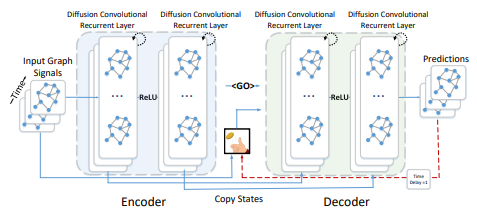
The spatial dependency is designed by concerning flow into a diffusion procedure that directly catches the traffic dynamics’ stochastic nature. The diffusion procedure will be considered as a haphazard walk upon G having a restart probability $\alpha \in[0,1]$ and a state transfer matrix $D_O^{-1} W$. In this, $D_O=$ $D I A G(W 1)$ indicates the out-degree diagonal matrix, and $1 \in$ $R^N$ indicates the entire 1 vector. Subsequent to several time phases, the Markov procedure converges toward an immobile dispensation $P \in$ $R^{N \times N}$ wherein $i^{\text {th }}$ row $P_i \in R^N$ portrays the diffusion similarity out of the node $v_i \in V$; thus, the proximity concerning the node $v_i$. Figure 2 shows Working of diffusion convolutional recurrent layer.
Figure 2. Working of diffusion convolutional recurrent layer
3.6 Diffusion convolution layer (DCL)
With the convolution procedure, we could construct a DCL, which maps P-dimensional features to Q-dimensional outputs. Indicate the criterion tensor as $\varphi \in R^{Q \times P \times K \times 2}=[\theta]_{q, p}, \ldots \in R^{K \times 2}$ that parameterizes the convolutional filter for the pth input and the qth output. The DCL, hence, remains:
$H_q=a\left(\sum_{p=1}^P X_p \times g f_{\theta q, p . \ldots}\right)$ for $q \in\{1,2, \ldots Q\}$
in which, $X \in R^{N \times P}$ denotes the input, $X \in R^{N \times Q}$ denotes the output, $f _{ \theta , p , \ldots}$ denotes the filters, and a denotes the activation function (for instance, ReLU, Sigmoid). DCL learns the portrayals for graph-structured data and could be trained by employing the stochastic gradient-related methodology. In betwixt succeeding encoder/decoder (E/D) units, a ReLU module (ReLUM) will be presented for lessening multi-scale features’ parallel connection. Same as the E/D unit, every ReLUM comprises multiple operational unit cells (UCs) functioning at disparate degrees. Let $F_i$ portrays the $i$ thReLUM, $F_{i, j}$ portrays the $i$ th UC of $j$ thReLUM in order that $=\{1,2,3, \ldots L\}$ (something is missing before the equal symbol), $j=\{1,2,3 \ldots 2 m-1\}$, and $F_{i, j} \in F_i$. Every ReLUM consumes entire feature portrayals' (FP) scales as input out of entire former $E / D$ phases, and produces L quantity of disparate FMs for the ensuing E/D phase via multi-scale features' (MSFs) deep fusion acquired out of the former phases. In every ReLUM's UC, an MSF collection strategy will be utilized that could be portrayed as $F_{i, j}=$ $f\left(E_1, E_2, \ldots E_{\frac{1}{2}}, D_1, D_{2,}, \ldots E_{\frac{1}{2}}\right.$, in which f(.) portrays the functional operations within the ReLU UC regarding the L scale of portrayals out of every former E/D unit. Out of the sequential decoder unit’s last level, multiple decoded FP will be acquired that will be processed collectively within the fusion optimizer (FO) module (O) for generating the last mask, and it could be presented as,
$O=f\left(D_{1,1}, D_{1,2}, \ldots D_{1,1}, D_{1, m}\right)$
in which, O(.) portrays the FO action. For managing the absence of contextual data (CDt) in the down-transitional procedure (TP), dense interconnection’s greater degree will be proffered amidst multi-scale FMs produced out of disparate UCs. In every unit, encoded FP produced out of entire UC’s greater degrees will be taken into consideration for producing down-scaled FM. Thus, the CD missed in every TP could be retrieved out of UC’s very deep stack as FP out of entire former cells that are regarding during transition. For converging multi-scale FMs out of former levels, initially, pooling procedures having disparate kernels will be performed for creating their spatial dimension uniform, and, consequently, channel-wise feature collection will be performed.
3.7 Diffusion sequential cell layer
For joining spatial and temporal designing, every matrix multiplication procedure will be substituted by the diffusion convolution procedure, explained in the former expression. The consequentialalteredsequential cell could be described as,
$r^{(t)}=\sigma\left(\theta_{r, G}\left[X^{(t)}, H^{(t-1)}\right]+b_r\right.$
$u^{(t)}=\sigma\left(\theta_{u, G}\left[X^{(t)}, H^{(t-1)}\right]+b_u\right.$
$C^{(t)}=\tanh \left(\theta_{C * G}\left[X^{(t)} ; r^{(t)} H^{(t-1)}\right]+b_c\right.$
$H^{(t)}=u^{(t)} \cdot H^{(t-1)}+\left(I-u^{(t)}\right) \cdot C^{(t)}$
in which, $X^{(t)}$ and $H^{(t)}$ indicate the input and output (or activation) at the time $t, r^{(t)}$ and $u^{(t)}$ indicate the reset gate and update gate, and $C^{(t)}$ indicates the candidate output that gives to the novel output centered upon the value of the updated gate $u^{(t)}$.
3.8 Prediction procedure
For reading intervals, this equalizes in predicting the subsequent [4, i, 12, 16,20, and 24 hours). There remain ceaseless amalgamations of input length T to prediction length (PL) N. The ensuing 4 input cases have been selected for this experiment.
Input Case 1: input T = 4, predict every N of NE
Input Case 1: input T = 12, predict every N of NE
Input Case 1: input T = 24, predict every N of NE
Input Case 2: input T = 48, predict every N of NE
Input Case 3: input T = 120, predict every N of NE
Input Case 4: input T = 288, predict every N of NE
The 6 input cases having 4 PLs create a sum of sixteen cases. Entire paradigms have been trained for ten epochs as this has been adequate for attaining a convergence’s acceptance level.
In this segment, we performed comprehensive simulations upon the LF jobs for authenticating that the proffered methodology could assist during the C-19P. Specifically, we correlated the proffered methodology with standard methodologies.
4.1 Dataset description
The load DSs have been gathered and built for diverse areas for analyzing the proffered LF technique. Particularly, hourly EC data for systems of disparate dimensions are employed: nation-level data of European nations (UK, Germany, and France), ISO-level data (CAISO, NYISO), zonal data in ERCOT (coastal, north-central, and south-central regions), and metropolitan-level data of the USA cities (Seattle, Chicago, Boston, the Mid-Atlantic region). The European LD have been gathered out of ENTSO-E, wherein the USA data remain publically accessible out of multiple ISO and partaking facilities. The entire gathered DSs will be present alongside the code repo for assessment. We question in any case forecast API World Weather Online and imply data normalization pre-processes every DS. For bigger load areas like CAISO and European nations, we sequence multiple main cities’ weather and motility data as the IF vectors. The 2 training DSs have been gathered for assessing the proffered technique. The initial DS omits motility features and covers the time range betwixt 01 Jan 2018 to 15 May 2020. The next DS employs accessible motility data ranging from 14 Feb 2020 to 15 May 2020 that remains a fairly little data for LF. Table 1. Load DSs’ assessment for prevailing methodologies. and Table 2. Error assessment for the proffered methodology concerning disparate areas.
4.2 Criteria
Mean Square Error (MSE) – This calculates the mean of the squares of errors or deviations. This as well indicates the second instant of error, which includes the estimator’s variance as well as bias.
$M S E=\frac{1}{n} \sum_{i=1}^n\left(x_i-y_i\right)^2$
Mean Absolute Percentage Error (MAPE) – This calculates the disparity betwixt 2 successive variables. For instance, variables y and x indicate the anticipated and noticed values and could be computed by,
$M A P E=\frac{100}{n} \sum_{i=1}^n \frac{\left(y_i-x_i\right)}{n}$
Root Mean Square Error (RMSE) – This remains the very typically employed measure for analyzing the prediction’s quality.
$R M S E=\sqrt{\frac{\sum_{i=1}^N\left(x_i-x_i^{\prime}\right)}{N}}$
Table 1. Load DSs' assessment for prevailing methodologies
|
Paradigm |
NN_Orig |
Retrain |
Mobi |
Mobi_MTL |
|
Seattle |
15.01 |
7.55 |
6.51 |
2.28 |
|
Chicago |
14.44 |
17.92 |
4.08 |
2.33 |
|
Boston |
6.55 |
15.6 |
4.38 |
2.91 |
|
Mid_Atlantic |
14.6 |
17.27 |
7.08 |
2.61 |
|
ERCOT_Coast |
7.38 |
7.17 |
1.85 |
1.8 |
|
ERCOT_NCENT |
8.48 |
9.6 |
2.7 |
1.59 |
|
ERCOT_SCENT |
8.16 |
7.73 |
5.18 |
2.71 |
|
NYISO |
12.91 |
15.55 |
6.25 |
5.24 |
|
CAISO |
8.51 |
7.77 |
5.97 |
3.15 |
|
UK |
10.11 |
13.78 |
8.74 |
4.46 |
|
GERMANY |
7.73 |
7.77 |
6.24 |
4.56 |
|
France |
22.71 |
8.31 |
5.93 |
4.1 |
Table 2. Error assessment for the proffered methodology concerning disparate areas
|
Area |
MSE |
MAPE |
MAE |
|
Seattle |
0.181 |
0.1691 |
0.0634 |
|
Chicago |
0.0534 |
0.2643 |
0.0935 |
|
Boston |
0.0429 |
0.3008 |
0.1155 |
|
Mid_Atlantic |
0.0578 |
0.3217 |
0.1828 |
|
ERCOT_Coast |
0.037 |
0.283 |
0.1505 |
|
ERCOT_NCENT |
0.071 |
0.4206 |
0.201 |
|
ERCOT_SCENT |
0.5883 |
0.6627 |
0.4748 |
|
NYISO |
0.0466 |
0.3183 |
0.1534 |
|
CAISO |
0.1024 |
0.5871 |
0.2216 |
|
UK |
0.5543 |
0.7487 |
0.5174 |
|
Germany |
0.0327 |
0.2089 |
0.1508 |
|
France |
0.0401 |
0.2513 |
0.1579 |
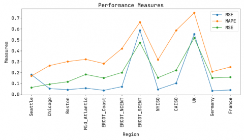
Figure 3. Error assessment for the proffered methodology
Figure 3 illustrates the errors’ assessment for the proffered DCRNN methodology in which the X-axis portrays diverse areas, and the Y-axis portrays the measures. The MSE has been assessed and the outcome has been acquired as: 0.181 for Seattle, 0.0534 for Chicago, 0.0429 for Boston, 0.0578 for Mid_Atlantic, 0.037 for ERCOT_Coast, 0.071 for ERCOT_NCENT, 0.5883 for ERCOT_SCENT, 0.0466 for NYISO, 0.1024 for CAISO, 0.5543 for the UK, 0.0327 for Germany, and 0.0401 for France. The MAPE has been assessed and the outcome has been acquired as: 0.1691 for Seattle, 0.2643 for Chicago, 0.3008 for Boston, 0.3217 for Mid_Atlantic, 0.283 for ERCOT_Coast, 0.4206 for ERCOT_NCENT, 0.6627 for ERCOT_SCENT, 0.3183 for NYISO, 0.5871 for CAISO, 0.7487 for the UK, 0.2089 for Germany, and 0.2513 for France. The MAE has been assessed and the outcome has been acquired as: 0.0634 for Seattle, 0.0935 for Chicago, 0.1155 for Boston, 0.1828 for Mid_Atlantic, 0.1505 for ERCOT_Coast, 0.201 for ERCOT_NCENT, 0.4748 for ERCOT_SCENT, 0.1534 for NYISO, 0.2216 for CAISO, 0.5174 for the UK, 0.1508 for Germany, and 0.1579 for France.
For giving supervision and citation for the PS’s EE scheduling and the shutdown and restart schedules of diverse firms during the C-19P, an LSTM paradigm through simplex optimizer has been developed for ELF. By correlating with the traditional LSTM paradigm and FC instance authentication for EL, the proffered DCRNN paradigm remains extremely appropriate for ELF bounded by the situations of the absence of training data samples, and optimum FC outcomes could be acquired by lesser training repetitions. This has been observed that the proffered DCRNN paradigm attains 0.0534 of MSE in the Chicago area, 0.1691 of MAPE in the Seattle area, and 0.0634 of MAE in the Seattle area. The prospective study would focus upon by regarding the rest of the TS data and analyze industrial implementations.
[1] Lu, R., Zhao, X., Li, J., et al. (2020). Genomic characterisation and epidemiology of 2019 novel coronavirus: implications for virus origins and receptor binding. Lancet, 395: 565-574. https://doi.org/10.1016/s0140-6736(20)30251-8
[2] Deif, M.A., Solyman, A.A.A., Hammam, R.E. (2021). ARIMA model estimation based on genetic algorithm for COVID-19 mortality rates. Int. J. Inf. Technol., pp: 1-24. https://doi.org/10.1142/S0219622021500528
[3] Wang, C., Horby, P.W., Hayden, F.G., Gao, G.F. (2020). A novel coronavirus outbreak of global health concern, Lancet, 395: 470-473.
[4] Deif, M., Hammam, R., Solyman, A. (2021). Adaptive neuro-fuzzy inference system (ANFIS) for rapid diagnosis of COVID-19 cases based on routine blood tests. Int. J. Intell. Eng. Syst.. https://doi.org/10.22266/IJIES2021.0430.16
[5] Rational use of personal protective equipment for coronavirus disease (COVID-19) and considerations during severe shortages: interim guidance, World Health Organization, 2020. https://iris.paho.org/handle/10665.2/51954, accessed on Sept. 17, 2022.
[6] Yy, S. (2020). Yang, Inhibition of SARS-CoV-2 replication by acidizing and RNA lyase-modified carbon nanotubes combined with photodynamic thermal effect. J. Explor. Res. Pharmacol., pp: 1-6. http://dx.doi.org/10.14218/JERP.2020.00005
[7] Pal, M., Berhanu, G., Desalegn, C., Kandi, V. (2020). Severe acute respiratory syndrome Coronavirus-2 (SARS-CoV-2): An update. Cureus, 12(3). https://doi.org/10.7759/cureus.7423
[8] Woo, P.C.Y., Huang, Y., Lau, S.K.P., Yuen, K.Y., Coronavirus genomics and bioinformatics analysis. Viruses, 2 (8), 1804-1820. https://doi.org/10.3390/v2081803
[9] Pachetti, M., Marini, B., Benedetti, F., Giudici, F., Mauro, E., et al. (2020). Emerging SARS-CoV2 mutation hot spots include a novel RNA-dependent-RNA polymerase variant. J. Transl. Med., 18: 1-9. https://doi.org/10.1186/s12967-020-02344-6
[10] Peñarrubia, L., Ruiz, M., Porco, R., Rao, S.N., Juanola-Falgarona, M., Manissero, D., López-Fontanals, M., Pareja, J. (2020). Multiple assays in a real-time RT-PCR SARS-CoV-2 panel can mitigate the risk of loss of sensitivity by new genomic variants during the COVID-19 outbreak. Int. J. Infect. Dis., 97: 225-229. https://doi.org/10.1016/j.ijid.2020.06.027
[11] Naeem, S.M., Mabrouk, M.S., Marzouk, S.Y., Eldosoky, M.A. (2020). A diagnostic genomic signal processing (GSP)-based system for automatic feature analysis and detection of COVID-19. Brief Bioinf. https://doi.org/10.1093%2Fbib%2Fbbaa170
[12] Deif, M., Hammam, R.E. Solyman, A. (2021). Gradient boosting machine based on PSO for prediction of Leukemia after a breast cancer diagnosis. Int. J. Adv. Sci. Eng, 11: 508-515. http://dx.doi.org/10.18517/ijaseit.11.2.12955
[13] Mikolov, T., Sutskever, I. Chen, K. Corrado, G.S., Dean, J. (2013). Distributed representations of words and phrases and their compositionality. Adv. Neural Inf. Process. Syst., 26: 3111-3119.
[14] Chaudhuri, A., Sahu, T.P. (2021). A hybrid feature selection method based on Binary Jaya algorithm for micro-array data classification. Computers &Electrical Engineering, 90(12).
[15] Wang, L., Gao, Y., Gao, S., Yong, X. (2021). A new feature selection method based on a self-variant genetic algorithm applied to Android malware detection. Symmetry, 13(7): 1290. http://dx.doi.org/10.3390/sym13071290
[16] Bae, J.H., Kim, M., Lim, J.S., Geem, Z.W. (2021). Feature selection for colon cancer detection using k-means clustering and modified harmony search algorithm. Mathematics, 9(5): 570. https://doi.org/10.3390/math9050570
[17] Al-Rajab, M., Lu, J., Xu, Q. (2021). A framework model using multifilter feature selection to enhance colon cancer classification. Plos one, 16(4): e0249094. https://doi.org/10.1371/journal.pone.0249094
[18] Liang, S., Mohanty, V., Dou, J., Miao, Q., Huang, Y., Müftüoğlu, M., Ding, L., Chen, K. (2021). Single-cell manifold-preserving feature selection for detecting rare cell populations. Nature Computational Science, 1(5): 374-384.
[19] Mock, F., Kretschmer, F., Kriese, A., Böcker, S., Marz, M. (2021). BERTax: taxonomic classification of DNA sequences with Deep Neural Networks. BioRxiv. http://dx.doi.org/10.1101/2021.07.09.451778
[20] Zhang, Y., Chen, Y., Bao, W., Cao, Y. (2021). A Hybrid Deep Neural Network for the Prediction of In-Vivo Protein-DNA Binding by Combining Multiple-Instance Learning. In International Conference on Intelligent Computing, Springer, Cham, pp. 374-384.
[21] Bukhari, S.A., Razzaq, A., Jabeen, J., Khan, S., Khan, Z. (2021). Deep-BSC: Predicting Raw DNA Binding Pattern in Arabidopsis thaliana. CurrentBioinformatics, 16(3): 457-465. http://dx.doi.org/10.2174/1574893615999200707142852
[22] Sanchez, T., Bray, E.M., Jobic, P., Guez, J., Charpiat, G., Cury, J., Jay, F. (2021). Dnadna: DEEP NEURAL ARCHITECTURES FOR DNA-A DEEP LEARNING FRAMEWORK FOR POPULATION GENETIC INFERENCE. https://hal.archives-ouvertes.fr/hal-03352910, accessed on Oct. 1, 2022.
[23] Sivangi, K.B., Dasari, C.M., Amilpur, S., Bhukya, R. (2022). NoAS-DS: Neural optimal architecture search for detection of diverse DNA signals. Neural Networks, 147: 63-71. https://doi.org/10.1016/j.neunet.2021.12.009
[24] Mehfooza, M., Pattabiraman, V. (2021). SP-DDPT: a simple prescriptive-based domain data preprocessing technique to support multilabel-multicriteria learning with expert information. International Journal of Computers and Applications, 43(4): 333-339. https://doi.org/10.1080/1206212X.2018.1547475
[25] Loshchilov, I., Hutter, F. (2016). SGDR: Stochastic Gradient Descent with Warm Restarts. ICLR 2017. https://doi.org/10.48550/arXiv.1608.03983
[26] Huang, G., Li, Y., Pleiss, G., Liu, Z., Hopcroft, J.E., Weinberger, K.Q. (2017). Snapshot Ensembles: Train 1, Get M for Free. ICLR 2017. arXiv 2017, arXiv:1704.00109.
[27] Gopi, A.P., Naik, K.J. (2021). A Model for Analysis of IoT based Aquarium Water Quality Data using CNN Model. In 2021 International Conference on Decision Aid Sciences and Application (DASA), pp. 976-980. http://dx.doi.org/10.1109/DASA53625.2021.9682251