Sheikh Amir Fayaz | Majid Zaman* | Sameer Kaul | Muheet Ahmed Butt
© 2022 IIETA. This article is published by IIETA and is licensed under the CC BY 4.0 license (http://creativecommons.org/licenses/by/4.0/).
OPEN ACCESS
When using machine learning to predict a class with a continuous numeric value, there are several issues. Only a few machine-learning approaches are capable of doing so, but it remains one of the most difficult jobs to do. In this paper, we show how to use the M5 Model Tree, an approach that can handle continuous numeric data. This method is a stepwise procedure that employs linear functions at the leaf nodes of any created decision tree inducer (such as CART). These M5 model trees provide basic practical formulas such as standard deviation (SD), standard deviation reduction (SDR), cost-complexity pruning (CCP), and so on, which may be simply applied to different benchmark data by another user. This study examines the M5 Model Tree algorithm's capabilities for analysing rainfall data in the Kashmir portion of India's Union Territory of Jammu & Kashmir. One of the best suited models was the M5 model tree, which was built using (70–30) percent training and test ratios, respectively, and predicted an RMSE of 2.593, an MAE of 1.68, and a correlation coefficient (R2) of 0.478. Furthermore, M5 model trees produce models with a minimal number of trails, requiring less computing effort and making them more practical to use.
regression, rainfall data, M5 model tree, smoothing, geographical data
For precise and methodical thinking in order to design future activities, real-time forecasts are essential. In order to create accurate and timely forecasts, the failure of present machine learning algorithms is a cause for concern. These early forecasts are critical for farmers, doctors, and others in fields such as agriculture, meteorology, and medicine [1]. Farmers worry that too much or too little rain may destroy their crops. It has impacted agricultural output in a number of arid and semiarid regions across the world, and it has emerged as one of humanity's most pressing challenges. Historical geographical characteristics such as vapor pressure, wind speed, humidity, temperature, density, and precipitation are utilized to determine future rainfall projections. Rainfall prediction has been done using a variety of soft computing methods [2]. Effective methods based on ANN and hybrid models have been used to predict rainfall in recent years. These technologies produce accurate and timely results, but their complicated designs are one of the major drawbacks of employing them. These models adopt a "black box" approach, in which the user can only assess the input and output numbers without knowing how the model works inside. On the rainfall data of Kashmir province, we evaluated the performance of an efficient M5 model tree technique, which is a stepwise approach that employs linear functions at the leaf nodes of any decision tree inducer (CART) produced [3]. Simple practical formulas such as standard deviation (SD), standard deviation reduction (SDR), cost-complexity pruning (CCP), and others are generated by these model trees, which may be readily applied by another user to different benchmark data. Furthermore, because model trees generate models using a small number of trails, they need less computing time and are thus much easier to utilize [4, 5].
Because of its lack of implementation in important programmes like Python and MATLAB, the M5 Model tree approach did not gain awareness across datasets. In this article, we used M5 Model tree to forecast rainfall using geographical data. When compared to other traditional and ensemble methodologies, the M5 Model tree's novelty is in its mathematical and analytical execution, which has delivered several enhanced outcomes.
In this research, we present a mathematical and analytical implementation of a theoretical M5 Model tree. Python and its various libraries were then implemented using Google Colaboratory. The pseudocode snippet is shown in the next section. The M5 Model tree was determined to perform better in terms of accuracy.
This paper is organised as follows: Section 1 provides a quick review of Model tree, M5 Model trees. Section 2 is a quick overview of the literature. In section 3, the material and dataset are described, while in section 4, the implementation of M5 model trees and a quick analysis of the findings are explained, as well as each attribute's unique prediction. Section 5 ends the paper.
1.1 M5 model tree
A model tree is a machine learning technique that works with numeric continuous objective values, and the M5 model tree is the learning algorithm that can deal with them. According to Quinlan's (1992) presentation, the M5 model tree technique combines any regular decision tree model with the probability of linear regression at the decision tree's leaf nodes. Because the decision tree looks to be a simple strategy, yet the regression function only has a few variables to work with [6].
The M5 model tree is built in two stages: a traditional decision tree and a linear regression function. To begin, the regression tree is constructed using the decision tree induction procedure. The standard deviation at each node will be determined to assess the predicted reduction in error for the splitting criterion. This node splitting in M5 will continue until there are very few instances left. Second, after constructing the normal regression tree, internal sub nodes are pruned and replaced with the regression plane rather than constant values. Pruning estimates the predicted error at each node [7].
Splitting takes a set, T, as input and divides it into smaller subsets, T1, T2, T3,...Tn. This is a recursive technique in which each sub-split is sub-split into offspring, and the process continues until there are very few instances remaining. At each internal node, this M5 employs a greedy approach to error minimization, with standard deviation reduction (SDR) determined one node at a time and provided by equation (1). A SDR is calculated at each node for splitting, and then cost complexity pruning (CCP), illustrated below (2), is applied at each leaf node to remove areas that may not be beneficial for the final tree, lowering the number of rules [8, 9].
$S D R=\frac{S D(T)-\sum S D\left(T_{i}\right)\left|T_{i}\right|}{|T|}$ (1)
$C C P=\frac{\operatorname{err}(\operatorname{prune}(T, t), S)-\operatorname{err}(T, S)}{\mid \text { leaves }(T)|-| \text { leaves }(\operatorname{prune}(T, t)) \mid}$ (2)
Smoothing is also conducted after pruning on the created Model Tree, which is used to prevent the harsh discontinuities of the sub trees. Flattening the sharp nodes of nearby models is a typical way to enhance prediction accuracy [10, 11].
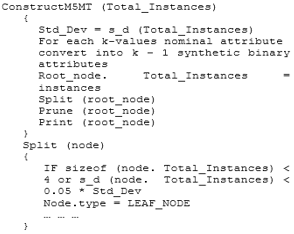
The split (Algorithm 1) and pruning (Algorithm 2) phases of the M5 model tree are specified in the code snippet algorithm (Pseudocode) shown below [12, 13].
Algorithm 1: Snapshot of M5 model tree approach with Split function
Because model trees are not as popular as other machine learning models. As a result, it has not been widely used, and very little work on M5 model trees has been done in the field of geographical sciences. During our literature search, we came across various studies in geographical sciences that used M5 model trees to conduct flood forecasting, calculating reference evapotranspiration, prediction of major wave height in Lake Superior, rainfall runoff modelling, and stream flow forecasting.
Algorithm 2: Snapshot of M5 model tree approach with prune & Error function
Fayaz et al. [14] provided a stepwise mathematical implementation of the logistic model tree (LMT), and the data for this study was acquired from the Indian Metrological Department (IMD) in Pune from 2012 to 2017, and it contains roughly 5580 records. Five factors make up the data, including humidity and temperature as independent variables and rainfall as the objective variable. The data utilized in the implementation process was discrete data, with the goal value depicting the presence or absence of rain. The model's accuracy statistics and various statistical measures were calculated, and the results were then compared to other traditional and ensemble models such as RF, DT, and DDT, with the logistic model tree outperforming these traditional and ensemble approaches.
Etemad-Shahidi and Mahjoobi [15] suggested a study in which the authors attempted to estimate major wave height in Lake Superior. This research uses Lake Superior wind and wave data from 2000 to 2001. The authors recommend M5 model trees over ANN because M5 model trees offer readily defined rules that humans can grasp. Furthermore, the findings show that M5 model tree error statistics were similar to those of ANN, although model trees were slightly more accurate.
Alipour et al. [16] used satellite pictures to calculate the reference evapotranspiration [ETo] estimate. This research was conducted at five Iranian weather stations. For the estimate, a basic linear regression with M5 model tree was created, and it performed better on the same set of data.
Nourani et al. [17] suggested a research based on the wavelet-M5 model tree for rainfall runoff modelling. The dataset was partitioned into three training and testing partitions (60-40 percent, 75-25 percent, and 50-50 percent, respectively), and the model was tested on daily and monthly rainfall scales. In both monthly and daily rainfall scales, the wavelet M5 model tree performs better, according to this study.
Solomatine and Xue [18] looked at an M5 model for flood forecasting in China. The M5 model trees and the ANN are compared head-to-head in this study, with both models accurately predicting high floods. Later on, a modular model based on a hybridization of the M5 and ANN models was created, which yielded the greatest prediction performance. Because this model is based on correlation analysis, it may be enhanced by adding hydrological information to refine the hydrological experts' inputs. As a result, utilizing the M5 model tree for classification, the supplied inputs will yield more hydrological features.
Some of the above literature studies of M5 model trees used in the geographical sciences are offered, however no study of M5 model trees used for rainfall prediction is presented. As a result, we conducted an experimental investigation of the M5 mode tree on rainfall data to see how accurate and practicable the model is [19-21]. This research will assist us in determining why this algorithm is not commonly used, as well as evaluating the performance of M5 mode tree on different types of data such as agricultural, health, and academic data [22, 23].
The table (Table 1) below shows a description of the data collected and the multiple parameters utilized for rainfall forecast in all zones of Kashmir province [18-21]. The final instances of the dataset comprise roughly 5500 elements after the preprocessing of the data.
The numerous relative values of the historical geographical parameters utilized in the study are shown in the graphical form in below. Figure 1 depicts relative frequency distributions as graphical representations. The key benefit of utilizing relative frequencies as characteristics is that it allows you to compare different frequencies of the individual attributes. The possibility or likelihood of receiving an observation from each category in a blind or random draw may be calculated using these relative frequencies. As a result, if we choose one observation at random, there's a good probability it'll be consistent across the dataset. As a result, a relative frequency distribution is frequently referred to as an empirical or observed probability distribution.
Figure 1. Graphical representations of relative values of geographical data
Creating a frequency distribution for a numeric variable is a little more challenging. Because few, if any, individual observations will have identical values, individual values of the variable being defined as categories will nearly always result in a list of the original observations. As a result, defining categories as value intervals known as class intervals is typical practice. The intervals must not overlap, and each class interval should be the same size in reference to the measuring scale.
Table 1. Dataset Description and Statistical properties with different parameters
|
Parameters |
Station No. |
Year |
Station Name |
Station Location |
Min |
Max |
Mean |
Std. Dev |
Variance |
Skewness |
Kurtosis |
|
Max Temp (°C) |
42026, 42027, 42044 |
2012-2017 |
South, North & Central Kashmir |
33.59°N 75.16°E, 34.05°N 74.38°E, 34.5°N 74.47°E |
-7.6 |
35.4 |
18.04 |
8.80 |
77.48 |
-0.24 |
-0.86 |
|
Min Temp (°C) |
-14.4 |
23.8 |
6.34 |
7.43 |
55.27 |
0.02 |
-0.84 |
||||
|
Humid12 (%) |
18 |
98 |
60.27 |
18.05 |
325.81 |
0.21 |
-0.73 |
||||
|
Humid3 (%) |
0 |
96 |
75.64 |
14.13 |
199.81 |
-0.76 |
0.39 |
||||
|
Rf (mm) |
0 |
206 |
2.75 |
9.07 |
82.25 |
7.74 |
99.39 |
We used the M5 Model tree technique on the dataset's 5 metrological parameters in this investigation. KNIME, an open source data analytics tool, was employed for the simulation investigation. The experiment was conducted on a 70-30 ratio, with 70% serving as the training set and 30% serving as the testing set. The dataset contains four independent continuous parameters: minimum and maximum temperatures, humidity at two different intervals, and a continuous dependent variable, rainfall [24, 25].
Following the evaluation of the data, multiple methodologies were used to examine the overall calculation of the data. The greatest number of rules generated using the Unsmoothed Unpruned M5 model tree was around 918, and when the pruning was applied and the smoothed linear model was used, the overall rules substantially decreased to 13 with little influence on performance, as shown in Table 2. The following is a clustered graphic that compares the number of rules in pruned and unpruned M5 linear models (Figure 2).
Table 2. M5 base model to check the number of rules
|
Model |
M5 Pruned Model Tree (Smoothed Linear Model) |
M5 Un-Pruned Model Tree (Un-Smoothed Linear Model) |
|
M5 Base Model Rules |
13 |
918 |
|
M5 Rules with M5 Pruned Model Rules Using Smoothed Linear Model |
10 |
111 |
|
M5 Rules with M5 Pruned Model Tree Using Un-Smoothed Linear Model |
16 |
100 |
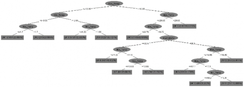
Figure 3 depicts the structure of the model tree discovered by M5 Model tree for the meteorological dataset of Kashmir province, using just 13 rules (LM 1 to LM 13) as leaves. The whole tree is given below, with the property Max Temp chosen as the parent node since it has the biggest information gain of all the attributes. This procedure is repeated until all of the nodes have been computed [26], and the resultant leaf nodes will have values for Linear model functions at each leaf node of the created tree.
Figure 2. Clustered chart to compare the number of rules data
Figure 3. M5 model tree stepwise construction
Table 3. Linear model Functions with Smoothed Linear models generated using M5Base model tree
|
Linear Models |
Rainfall Statistics |
|
Linear Model_1 |
-1.41 x [Param_1] + 1.87 x [Param_2] + 0.02 x [Param_3] - 0.10 x [Param_4] + 21.20 |
|
Linear Model _2 |
-0.33 x [Param_1] + 0.15 x [Param_2] + 0.02 x [Param_3] - 0.03 x [Param_4] + 4.60 |
|
Linear Model _3 |
-1.86 x [Param_1] + 1.02 x [Param_2] + 0.20 x [Param_3] - 0.51 x [Param_4] + 44.51 |
|
Linear Model _4 |
-2.02 x [Param_1] + 6.10 x [Param_2] + 1.51 x [Param_3] - 2.10 x [Param_4] + 74.61 |
|
Linear Model _5 |
-0.25 x [Param_1] + 0.41 x [Param_2] + 0.01 x [Param_3] - 0.02 x [Param_4] + 4.71 |
|
Linear Model _6 |
-1.41 x [Param_1] + 0.91 x [Param_2] + 0.35 x [Param_3] - 0.54 x [Param_4] + 45.90 |
|
Linear Model _7 |
-2.42 x [Param_1] + 2.25 x [Param_2] + 0.51 x [Param_3] - 0.80 x [Param_4] + 60.48 |
|
Linear Model _8 |
-1.86 x [Param_1] + 2.78 x [Param_2] + 0.51 x [Param_3] - 0.81 x [Param_4] + 38.22 |
|
Linear Model _9 |
-2.81 x [Param_1] + 0.60 x [Param_2] + 0.13 x [Param_3] - 0.37x [Param_4] + 66.02 |
|
Linear Model _10 |
-0.55 x [Param_1] + 0.82 x [Param_2] + 0.22 x [Param_3] - 0.66 x [Param_4] + 45.02 |
|
Linear Model _11 |
-0.55 x [Param_1] + 0.90 x [Param_2] + 0.28 x [Param_3] - 0.82 x [Param_4] + 57.05 |
|
Linear Model _12 |
0.61 x [Param_1] + 0.27 x [Param_2] + 0.02 x [Param_3] - 0.14 x [Param_4] - 3.50 |
|
Linear Model _13 |
-0.22 x [Param_1] + 0.19 x [Param_2] - 0.019 x [Param_3] - 0.01 x [Param_4] + 5.80 |
|
where, Param_1 à [Minimum Temperature] Param_2 à [Maximum Temperature] Param_3 à [Humidity 12pm] Param_4 à [Humidity 3am] |
|
Table 3 illustrates Linear Model functions for rainfall generated using M5 Base Model Tree with Smoothed Linear models.
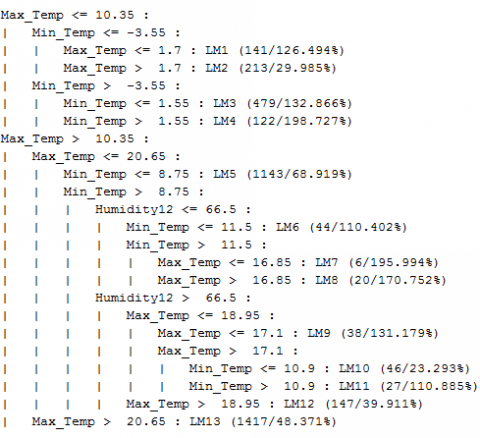
Figure 4 shows a screenshot of the section of rules created by the M5 Model tree method. These created rules follow the IF-then ELSE criteria, where all the attributes are analyzed and the root node is chosen based on the maximum information gain, and the process proceeds to produce the leaf node with values (Linear Model_1 through Linear Model_13 Linear model functions).
Figure 4. Generation of rules using M5 model tree algorithm
Since the major goal of this study was to analyze data using the M5 model tree approach, it was discovered that continuous target values may be studied more successfully than normal regression. Because when the regression tree is taken into account, the size of the M5 model created is relatively little. In a normal regression, the number of rules is equal to the total number of occurrences of the target variable, but in M5 model trees, the number of rules may be counted [27, 28].
The M5 model tree was applied to the same historical Geographical data for rainfall prediction, and the correlation coefficient was computed as shown in table (Table 4):
Table 4. Accuracy statistics
|
Statistics |
Value |
|
R2 |
0.478 |
|
Mean absolute error |
1.689 |
|
Mean Squared error |
6.726 |
|
Root mean squared error |
2.593 |
|
Mean signed difference |
0.844 |
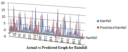
Figure 5. Actual vs Predicted Graphs for the rainfall parameter using M5 model tree algorithm
The snapshot (Figure 5) above shows the actual and expected values for rainfall parameter generated from the M5 model.
Numerous scholars from throughout the world have attempted to predict rainfall, with variable results. Various methods, such as NARX and ANN models, are examples of recent advances. In order to improve on the literature ideas, Onyari and Ilunga [29] conclude in their study that M5 Model tree produces better outcomes than ANN-MLP. As a result, a mathematical framework was created and constructed for its implementation on Google Colab.
On the geographical dataset, the final accuracy statistics of the M5 Model tree offer astounding results, with the maximum accuracy measure obtained by any conventional or ensemble technique on the same amount of data [30].
Since then, we've statistically implemented M5 Model tress for rainfall prediction, and the consequences demonstrate a significant improvement in performance when compared to classical and ensemble techniques on the same set of data. However, the influence of M5 Model trees on other datasets was not investigated in this study. The findings in this work are inevitably restricted, and they do not account for several other research trends. As a result, it is strongly advised that the same implementation be tested on several datasets. Furthermore, scientific studies where M5 Model trees have been utilized for prediction purposes are not available, preventing us from comparing M5 models.
By applying the heuristic approach technique to build the series of linear models functions at each leaf node of the tree, this work primarily focuses on the production of rules from numeric predictions of continuous data. It explains how classification and regression issues may be turned into more common linear model function approximations. The major goal of this research was to analyze data using the M5 model tree technique, and it was discovered that continuous target values may be examined more successfully than normal regression models. Because when the regression tree is taken into account, the size of the M5 model created is relatively little. In a normal regression, the number of rules is equal to the total number of occurrences of the target variable, but in M5 model trees, the number of rules is countable. The M5 model tree outperforms the normal regression tree by having nearly 5 times fewer rules, lowering the size of the tree without hurting overall performance and allowing for the use of local linearity in the data. The M5 model trees' trimmed and smoothed findings suggest a subsequent rise in prediction accuracy. Smoothing, on the other hand, may often increase the complexity of linear models, making it difficult to examine forecast accuracies. The M5 model tree, which was built using (70-30) percent training and test ratios, was found to be one of the best fit models, predicting RMSE of 2.593, MAE of 1.68, and correlation coefficient (R2) of 0.478. One of the key advantages of M5 mode trees over traditional regression trees is that traditional regression trees can never predict values outside the range of the trained model, but M5 model trees can extrapolate.
There is currently no approach that can simplify the heuristic functions at the leaf nodes, which are always a compromise between pruning factor and tree size, and this has to be corrected further. In addition, the computational cost of the M5 unpruned model tree should be explored. The multiple input and single output (MISO) models were investigated in this study. We can also assess performance using the multiple inputs and multiple outputs (MIMO) paradigm in the future.
[1] Kaya, Y.Z., Üneş, F., Demirci, M., Taşar, B., Varçin, H. (2018). Groundwater level prediction using artificial neural network and M5 tree models. Aerul si Apa. Componente ale Mediului, 195-201.
[2] Bahmani, R., Solgi, A., Ouarda, T.B. (2020). Groundwater level simulation using gene expression programming and M5 model tree combined with wavelet transform. Hydrological Sciences Journal, 65(8): 1430-1442. https://doi.org/10.1080/02626667.2020.1749762
[3] Rezaie-Balf, M., Naganna, S.R., Ghaemi, A., Deka, P.C. (2017). Wavelet coupled MARS and M5 Model Tree approaches for groundwater level forecasting. Journal of Hydrology, 553: 356-373. https://doi.org/10.1016/j.jhydrol.2017.08.006
[4] Adnan, R.M., Petroselli, A., Heddam, S., Santos, C.A.G., Kisi, O. (2021). Comparison of different methodologies for rainfall–runoff modeling: Machine learning vs conceptual approach. Natural Hazards, 105(3): 2987-3011. https://doi.org/10.1007/s11069-020-04438-2
[5] Nourani, V., Davanlou Tajbakhsh, A., Molajou, A., Gokcekus, H. (2019). Hybrid wavelet-M5 model tree for rainfall-runoff modeling. Journal of Hydrologic Engineering, 24(5): 04019012. https://doi.org/10.1061/%28ASCE%29HE.1943-5584.0001777
[6] Fayaz, S.A., Zaman, M., Butt, M.A. (2022). Numerical and experimental investigation of meteorological data using adaptive linear m5 model tree for the prediction of rainfall. Review of Computer Engineering Research, 9(1): 1-12. https://doi.org/10.18488/76.v9i1.2961
[7] Quinlan, J.R. (1992). Learning with continuous classes. In 5th Australian Joint Conference on Artificial Intelligence, 92: 343-348. https://doi.org/10.1142/9789814536271
[8] Landwehr, N., Hall, M., Frank, E. (2005). Logistic model trees. Machine Learning, 59(1-2): 161-205. https://doi.org/10.1007/s10994-005-0466-3
[9] Frank, E., Wang, Y., Inglis, S., Holmes, G., Witten, I.H. (1998). Using model trees for classification. Machine Learning, 32(1): 63-76. https://doi.org/10.1023/A:1007421302149
[10] Sidiq, S.J., Zaman, M., Ahmed, M. (2019). How machine learning is redefining geographical science: A review of literature. International Journal of Emerging Technologies and Innovative Research, 6: 1731-1746.
[11] Fayaz, S.A., Zaman, M., Butt, M.A. (2022). Knowledge discovery in geographical sciences—A systematic survey of various machine learning algorithms for rainfall prediction. In International Conference on Innovative Computing and Communications, pp. 593-608. https://doi.org/10.1007/978-981-16-2597-8_51
[12] Zaman, M., Butt, M.A. (2012). Information translation: A practitioners approach. In World Congress on Engineering and Computer Science (WCECS), Vol I, San Francisco, USA.
[13] Fayaz, S.A., Altaf, I., Khan, A.N., Wani, Z.H. (2019). A possible solution to grid security issue using authentication: An overview. Journal of Web Engineering & Technology, 5(3): 10-14.
[14] Fayaz, S.A., Zaman, M., Butt, M.A. (2021). An application of logistic model tree (LMT) algorithm to ameliorate prediction accuracy of meteorological data. International Journal of Advanced Technology and Engineering Exploration, 8(84): 1424-1440. https://doi.org/10.19101/IJATEE.2021.874586
[15] Etemad-Shahidi, A., Mahjoobi, J. (2009). Comparison between M5′ model tree and neural networks for prediction of significant wave height in Lake Superior. Ocean Engineering, 36(15-16): 1175-1181. https://doi.org/10.1016/j.oceaneng.2009.08.008
[16] Alipour, A., Yarahmadi, J., Mahdavi, M. (2014). Comparative study of M5 model tree and artificial neural network in estimating reference evapotranspiration using MODIS products. Journal of Climatology.
[17] Nourani, V., Davanlou Tajbakhsh, A., Molajou, A., Gokcekus, H. (2019). Hybrid wavelet-M5 model tree for rainfall-runoff modeling. Journal of Hydrologic Engineering, 24(5): 04019012.
[18] Solomatine, D.P., Xue, Y. (2004). M5 model trees and neural networks: Application to flood forecasting in the upper reach of the Huai River in China. Journal of Hydrologic Engineering, 9(6): 491-501.
[19] Kaul, S., Fayaz, S.A., Zaman, M. and Butt, M.A. (2022). Is decision tree obsolete in its original form? A burning debate. Revue d'Intelligence Artificielle, 36(1): 105-113. https://doi.org/10.18280/ria.360112
[20] Fayaz, S.A., Kaul, S., Zaman, M., Butt, M.A. (2022). An adaptive gradient boosting model for the prediction of rainfall using ID3 as a base estimator. Revue d'Intelligence Artificielle, 36(2): 241-250. https://doi.org/10.18280/ria.360208
[21] Fayaz, S.A., Zaman, M., Butt, M.A. (2021). To ameliorate classification accuracy using ensemble distributed decision tree (DDT) vote approach: An empirical discourse of geographical data mining. Procedia Computer Science, 184: 935-940. https://doi.org/10.1016/j.procs.2021.03.116
[22] Fayaz, S.A., Zaman, M., Butt, M.A. (2022). A hybrid adaptive grey wolf Levenberg-Marquardt (GWLM) and nonlinear autoregressive with exogenous input (NARX) neural network model for the prediction of rainfall. International Journal of Advanced Technology and Engineering Exploration, 9(89): 509. https://doi.org/10.19101/IJATEE.2021.874647
[23] Fayaz, S.A., Zaman, M., Kaul, S., Butt, M.A. (2022). Is deep learning on tabular data enough? An assessment. International Journal of Advanced Computer Science and Applications, 13(4): 466-473. https://doi.org/10.14569/IJACSA.2022.0130454
[24] Zaman, M., Kaul, S., Ahmed, M. (2020). Analytical comparison between the information gain and Gini index using historical geographical data. International Journal of Advanced Computer Science and Applications, 11(5). https://doi.org/10.14569/IJACSA.2020.0110557
[25] Ashraf, M., Zaman, M., Ahmed, M. (2018). Performance analysis and different subject combinations: An empirical and analytical discourse of educational data mining. In 2018 8th International Conference on Cloud Computing, Data Science & Engineering (Confluence), pp. 287-292. https://doi.org/10.1109/CONFLUENCE.2018.8442633
[26] Fayaz, S.A., Zaman, M., Butt, M.A. (2022). Performance evaluation of GINI index and information gain criteria on geographical data: An empirical study based on JAVA and Python. In International Conference on Innovative Computing and Communications, pp. 249-265. https://doi.org/10.1007/978-981-16-3071-2_22
[27] Altaf, I., Butt, M.A., Zaman, M. (2022). Disease detection and prediction using the liver function test data: A review of machine learning algorithms. In International Conference on Innovative Computing and Communications, pp. 785-800. https://doi.org/10.1007/978-981-16-2597-8_68
[28] Altaf, I., Butt, M.A., Zaman, M. (2021). A pragmatic comparison of supervised machine learning classifiers for disease diagnosis. In 2021 Third International Conference on Inventive Research in Computing Applications (ICIRCA), pp. 1515-1520. https://doi.org/10.1109/ICIRCA51532.2021.9544582
[29] Onyari, E.K., Ilunga, F.M. (2013). Application of MLP neural network and M5P model tree in predicting streamflow: A case study of Luvuvhu catchment, South Africa. International Journal of Innovation, Management and Technology, 4(1): 11-15. https://doi.org/10.7763/IJIMT.2013.V4.347
[30] Mohd, R., Butt, M.A., Baba, M.Z. (2020). GWLM–NARX: Grey Wolf Levenberg–Marquardt-based neural network for rainfall prediction. Data Technologies and Applications, 54(1): 85-102. https://doi.org/10.1108/DTA-08-2019-0130