Marin Mandić* | Goran Kraljević
© 2022 IIETA. This article is published by IIETA and is licensed under the CC BY 4.0 license (http://creativecommons.org/licenses/by/4.0/).
OPEN ACCESS
Due to strong competition in the telecom market, telecom companies are facing customer churn problems. For telecom, it is very important to predict the churn of a user to be able to prevent it. Marketing campaigns can be used to prevent churn and thus prevent a decrease in revenue. Usually, the churn prediction is based on behavioural user data, which describes user activity and general user data. In our prediction model, we added social network attributes that describe the social influence of other users on the user's decision to make a churn. Besides standard centrality measures, we developed two new social attributes, which measure the social influence of already churned users. To determine if social network attributes aid in churn prediction precision we created and compared the models based only on the behavioural data and the models with the social attributes and behavioural data. In our work, we propose upgrading the standard Automated Machine Learning (AutoML) model with the part of the model related to Social Network Analysis (SNA), and we use the proposed model in our research. We show that the AutoML can be used to successfully predict telecom churn based on the real data from telecom operators from Bosnia and Herzegovina.
AutoML, churn influence of a neighbour, prediction modelling, social network analysis (SNA), Telcom prepaid churn
This paper deals with the telecom churn problem for prepaid users using real data from telecom operator from Bosnia and Herzegovina. The telecom market in Bosnia and Herzegovina is very competitive, so users have the option of choosing another operator and better tariff offers. The ease of switching to another operator while maintaining the existing number encourages users to search for a better offer. The telecom companies are losing 20% to 40% of their users each year [1]. In their work, Lazarov and Capota [2] had shown that it is five to six times more expensive to bring in a new user than to keep an existing one. That fact shows how important churn management is. In order to effectively manage user churn, it is crucial to build a more effective and accurate churn prediction model. The Churn prediction model produces a list of users with a high probability of churn. This list is used in marketing campaigns designed to retain potential churners. A marketing campaign has to be harmonized with the customer experience strategy. Managing a good customer experience is valued by the customer and that is an additional way to retain existing customers. Customer experience is defined as the sum of all experiences that a customer has at every touch-point of the customer-company relationship [3].
The telecom users communicate with other telecom users using voice and messaging services. In this way, they make connections and build communities among themselves. Those communications between the users can be detected by using a call detail record (CDR) in the telecom billing system. By using the telecom CDRs it is possible to create a Social Network Analysis (SNA) and extract knowledge from those data. User decision to churn can be influenced by the user’s friends and family. Therefore, we use the SNA attributes to see will they improve churn prediction. The strength of the influence of friends is not the same, so we measured the importance of every user and used this measurement in developing models. In this paper, we create a telecom social network using a graph database and calculate seven SNA measures from the created social network. We will develop two models for predicting telecom churn, one model will use only traditional attributes (behavioural data and general user data), the second model will use traditional and SNA measures to predict churn. Models will be developed using Automated Machine Learning (AutoML). For developed models, we will verify whether it is valuable to use the SNA attributes to improve the precision.
This paper is organized as follows: Section 2 describes previous research of churn prediction in the telecom industry, social network analysis and AutoML. Section 3 demonstrates model creation, data preparation and experiment. Section 4 presents results and interpretation of the result, while Section 5 presents the conclusion.
2.1 Churn prediction in telecom
Telecom companies use machine learning for different purposes such as churn prediction, fraud detection, developing new products, customer segmentation etc. The first step in churn prediction process is data gathering. Historical data on user behaviour is needed to be able to predict future user behaviour. The input data set needs to be prepared in order to develop a successful churn prediction model. A common problem with the input data sat is data imbalance, taking into account the target variable. A group of authors described in their paper [4] ways to solve the problem of class imbalance. Data preparation includes data normalization [5], derivation of variables [6], feature selection [7-9] and noise removal [9].
Different machine learning algorithms can be used to predict churn such as: Decision Tree [5-8], Neural Networks [5, 6], Logistic regression [5, 7, 9, 10], Naive Bayes [9], Support Vector Machine [7, 11, 12], Random Forest [7-9, 12], Gradient Boosted Trees [7, 8, 10], Deep Learning [10, 13, 14], ensemble methods [12] etc. A mechanism for testing the validity of the developed telecom prediction model should also be established. This can be done by dividing the data into training and test set [6] and using k-fold cross validation [5, 7, 8].
2.2 Social network analysis (SNA)
SNA is a set of analytic methods used to show and measure connectivity and interaction between people, groups, organizations, computers and other connectable entities [15]. Common usage of an SNA in the telecom industry involves the identification of the most influential users in the telecom network [16], the identification of communities and groups [17], fraud detection [18], tariff model recommendation system [19] and predicting telecom churn [8, 20-22].
A group of authors in their work [8] extracted SNA measures from data and created a telecom churn prediction model using those measures. Due to the large amount of data model developed in this work uses machine learning techniques on the big data platform. They demonstrated that using SNA enhanced the performance of the churn prediction model.
Pushpa [20] developed the multi-relational social network based on relation type. They extract the hidden communities of the churners and non-churners from multi-relational SNA.
In their work, Gamulin et al. [21] used only SNA attributes to make churn predictions. They showed that the performance of the model was approximately the same when using a single SNA variable as in cases using two or three variables. They also observed that the user's churn depends on the previous behaviour of his neighbours.
Kostic et al. [22] created a churn prediction model using SNA in combination with clustering. They identified some important nodes in the telecom social network that are vital regarding churn prediction.
2.3 Automated machine learning (AutoML)
Developing machine learning models requires a lot of manual work, knowledge of the problem domain and expert knowledge in the development of machine learning applications [10]. AutoML helps experts to automate a manual repetitive task in the process of developing models. AutoML is defined as “software capable of being trained and tested without human intervention” [23].
AutoML is used to automate the following steps of developing machine learning applications: data preparing, model selection, hyperparameter optimization and meta-learning. In the past couple of years, AutoML gained a lot of focus. Therefore, various research papers and many different tools and platforms are dealing with AutoML.
Data preparation takes a lot of manual work and it is estimated that it is the most time-consuming step that usually takes up 50-70% of project time [24]. Using AutoML it is possible to get rid of repetitive manual data task like data cleaning, attribute selection, attribute generation, binning, attribute normalization etc.
The Combined Algorithm Selection and Hyperparameter Optimization (CASH) problem is the most important part of AutoML and it has been formulated by Auto-WEKA [25]. CASH automatically chooses an algorithm and its hyper-parameters for a given dataset and in some AutoML tools enable an analysis of developed models.
Meta-learning [26] is the concept to optimize the learning process based on previous experience in a data-driven way.
A group of authors in their work propose an automated and distributed ML framework and test it using real telecommunication data in several use cases [27]. Their proposed Auto ML framework does not contain SNA.
Mandic and Kraljevic [10] introduce a two-layer architecture that automates self-repairing of the churn prediction model. AutoML solution in this work reduces the time needed for developing models so it is possible to exclude the implementation window. As far as we know, previous works in the field of Auto-ML do not take into account SNA, which is the motivation for our work.
To be able to make a successful telco churn prediction we propose creating the following model as shown in Figure 1. We propose upgrading the standard AutoML model with the part of the model related to SNA, i.e. Social Network construction and Calculation of SNA measures. In the first step, the data is collected from the source system and prepared for the next steps. The input data is sent to two data streams, one to construct the social network and the other to the AutoML section. Creating telco SNA is a prerequisite for the calculation of SNA measures. The calculated SNA measures are sent to the AutoML section to improve the precision of the churn prediction model. The central part of the model is the Auto ML section where RapidMiner AutoML automatically prepares data, selects algorithms and makes hyperparameter tuning. After creating the model, the model needs to be tested and validated. If the created model has good precision, then it is possible to move on to the last step which is deployment. Created model is used in this work to create telco churn predictions using real telco data.
Figure 1. Model of creating telco churn prediction using AutoML with SNA
3.1 Preparing data
In this section, we will explain the data preparation and experiment which we made. Input data used in this experiment has 50.717 records. The number of users indicated as churners are 6.217, which means there are 12.26% of the churners.
We used four months of behavioural user data extracted from the CDR (Call Details Records) and one month of user churn. Trend attributes have been calculated using behavioural period. First, we calculate the average of the three periods (2019-07, 2019-08 and 2019-09). Then we calculate the difference between the period that precedes the churn period (2019-10) and a calculated average of the three preceding periods. The data time frame is shown in Figure 2.
Figure 2. Data time frame [10]
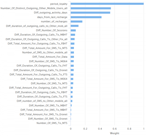
We created initial input data set that has 148 attributes based on user activity and general user data. The RapidMiner AutoML suggests that 120 attributes should be removed from the data set due to their poor quality. RapidMiner shows that attributes should be removed because of correlation, ID-ness, stability, missing values and text-ness. Additionally, we calculate the relevance of the remaining 28 attributes by computing the value of correlation for each attribute of the input data set concerning the churn attribute. We get the graph of the attribute weight in Figure 3. We have selected attributes with a weight greater than 0.07 in this way we get 7 behavioural and general attributes. Three trend attributes were selected for modelling.
They are calculated as the difference between the periods that precede churn period and calculated the average of preceding periods:
diff number of sessions;
diff outgoing activity days;
diff duration of outgoing calls to other mobs.
Figure 3. Attribute weight
In our experiment we also use the behavioural attributes from a period that precedes the churn period (2019-10):
number of distinct outgoing other mobile users;
days from the last recharge;
number of recharges.
Because we are doing an experiment based on prepaid data we do not have general user data like age, gender etc. The only general attribute that we use in this experiment is:
period loyalty.
Attribute period loyalty describes how long the user consumes the telecom services and therefore this attribute defines user loyalty as an important attribute for predicting telecom churn. A group of authors in their paper [28] described that the greater the loyalty of users, the better the stability of users and the less likely users are to churn.
3.2 Creating telco SNA using a graph database
Three months of CDR data and 43 million records have been used to create a telecom social network. It is possible to calculate SNA measures that describe the network as a whole and measures intended to determine the position of an individual node within the network. In our work, we calculate measures concerning an individual node.
We base our social network on the interactions between telecom users using call and messaging services. In our developed model, we give equal importance to one message and one minute of call. Because of computational reasons, we reduced the number of records by summing the minutes of calls and number of sent messages and by that we calculate connection weight between users. In this way, we created an edge list that is needed to create a social network. The commonly social network can be created using data located in the adjacency matrix or the edge list. Table 1 shows a part of the created edge list, which contains nodes in the first two columns. A pair of nodes in the same line indicates that these nodes are connected. Weight column in the edge list describes the strength of the connection (sum of sent messages and the duration of the call in minutes during the three months). The data used to create an edge list is anonymized. We also created a list of distinct users that are going to become nodes in SNA.
In the next step, we import nodes and relations in the most popular graph database Neo4j that we used because of performance reasons. Neo4j is a graph database management system that uses graph structure as its storage structure. Neo4j consists of nodes, relationships and attributes. Using the Neo4j graph database we can quickly query node related information through deep traversal and other methods [29].
Table 1. Edge list
|
Number A |
Number B |
Weight |
|
159207 |
384338 |
63,30 |
|
308494 |
385417 |
8,03 |
|
164105 |
386803 |
3,60 |
|
113642 |
387721 |
7,33 |
|
381835 |
387789 |
26,83 |
|
384995 |
388886 |
24,97 |
|
181668 |
391315 |
2,50 |
An important feature of graph databases is that it provides native processing capabilities, at least a property called index-free adjacency, meaning that every node is directly linked to its neighbour node [30]. Because of this graph database concept, it reduces the number of joins, reduces the number of data access, and therefore has very good performance. For selecting and manipulating data from the Neo4j database we use a cypher, the property graph query language which has been originally designed and implemented in the Neo4j graph database. Using Neo4j and Cypher query we can easily view relations between users in a graphical way.
Figure 4. Graphic representation of telecom social network
When visualizing a larger social network, there are problems with too many nodes to display, positioning nodes and unclear visualizations of connections between nodes. Because of that in Figure 4 we displayed only a small subset of created network. Created network show nodes that are connected directly and indirectly with a node with id 1616. Nodes that already had been churned are marked with red colour. Values in the red bubbles mark the calculated centrality measure from that node. Nodes that have high centrality measures have a high influence on neighbour’s nodes. From Figure 4 it can be seen that node 1616 has one directly connected churner with an influence strength of 1.2. It can also be seen that node 1616 has one indirectly connected churner with an influence strength of 1.1. We can see that the influence coefficient on node 1616 of directly connected users is 1.2 and 1.1 of indirectly connected users. A detailed explanation of how the influence attributes of neighbours who are already churned are calculated is shown in the next section.
3.3 Calculation of SNA measures
It is possible to calculate various centrality measures that can help us in the analysis of social networks. In our work, which is based on created telecom social network graph, we calculate the following measures:
degree centrality;
closeness centrality;
betweenness centrality;
eigenvector centrality;
article rank;
churn influence of neighbour distance one (CIONDO);
churn influence of neighbour distance two (CIONDT).
Degree centrality is measured by the node's total amount of direct links with the other nodes, based on the standardized formula CD (1) shown in [31].
$C_{D}\left(n_{i}\right)=\frac{d\left(n_{i}\right)}{g-1}$ (1)
where, d(ni) is degree of node, g is group size $n i \in V$ and the V is the set of nodes.
Degree centrality determines an importance score of a node based on the number of links held by each node. By calculating degree centrality it is possible to answer how many people this person can reach directly.
Closeness centrality measure shows how close a node is to all the other nodes. Nodes with a high closeness measure value have the shortest distances to all other nodes and because of that can spread information very efficiently through a graph. Beauchamp in his work [32] suggests multiplying Cc by (n-1) so that we could get the standardized equation, as shown in formula (2).
$C_{C}^{\prime}($ ni $)=\frac{n-1}{\left[\sum_{j=a}^{n} d(n i, n j)\right]}$ (2)
where, n stands for total number of nodes in network, and $\sum_{j=a}^{n} d(n i, n j)$ means the total number of steps from node N to the other nodes in the network.
Betweenness centrality is a measure used to detect the amount of influence a node has over the flow of information in a graph and to find nodes that serve as a bridge from one part of a graph to another. Let gjk be the number of shortest paths from node j to node k, gjk(ni) is the number of those paths that pass through node i. The node betweenness index for n is the sum of these estimated probabilities over all pairs of nodes not including the i-th node as shown in (3) by authors Wasserman and Faust [31].
$C_{B}\left(n_{i}\right)=\sum_{j<k} \frac{g_{j k}\left(n_{i}\right)}{g_{j k}}$ (3)
The betweenness may be normalized by dividing through the number of pairs of nodes not including ni, which for directed graphs is (g−1)(g−2) and for undirected graphs is (g−1)(g−2)/2.
Eigenvector centrality measures the transitive influence or connectivity of nodes and in this way answers how well is node connected to another well-connected node. In eigenvector centrality, connection to other nodes does not have the same importance. Connection to influential nodes contributes more to the eigenvector centrality value of a node than connections to low-scoring nodes. Eigenvector centrality measure is calculated by the formula (4) as shown in [33].
$X_{v}=\frac{1}{\lambda} \sum_{t \in M(v)} x_{t}$ (4)
where, M(v) is the set of the neighbours of node v, xt is centrality score of node $t$ and $\lambda$ is a constant.
ArticleRank is a variant of the Google’s Page Rank algorithm, which measures the influence of nodes. Article rank formula (5) is shown in the paper [34].
ArticleRank $(A)=1-d+d \times \overline{N R} \times\sum_{i=1}^{n} \frac{\text { ArticleRank }\left(P_{i}\right)}{\overline{N R}+N R\left(P_{i}\right)}$ (5)
where, ArticleRank(A) denotes the ArticleRank score of a node A, d is a damping factor set to 0.85, Pi (1<=I<=n) is one of the n nodes that is connected to the node A, $\overline{N R}$ is mean value of NR and NR(Pi) is the number of connections for Pi in the telecom social network.
Each user can be influenced by the users he is connected to. The user also influences other users, and consequently, he can influence the future behaviour of other users. This kind of influence between users is very important for telecom companies, since telecoms find a very important fact that the user will stop using their services and change the telecom operator [15]. We assume that an already churned user can influence his neighbour’s and neighbour neighbour’s decision to churn.
Gamulin et al. [21] created a social network measure of the relative number of neighbours who had already churned.
We also create two additional social network measures based on the importance of influence but with differences from the measure created in Ref. [21].
The first measure that we develop is Churn Influence of Neighbour Distance One (CIONDO), which calculates how many directly connected users have been churned in the previous period. Directly connected users are users whose mutual distance length is one. The distance dij between two users i and j is the number of edges along the shortest path connecting them. Not all nodes have the same influence on other nodes. Because of that fact, we calculate the centrality measures of nodes to determine the influential power of every node. For each node that already has been churned, we calculate betweenness and degree measures. Centrality measures have a large scale of values so we normalize those measures using range normalization with defined boundaries between 1 and 3.
In that way, we calculated the influence coefficient InfKoef of every already churned node. We propose the formula for calculating CIONDO measure and it is given in (6).
CIONDO $=\sum_{i=1}^{n} d\left(n c_{i}\right) \times \operatorname{InfKoef}$ (6)
where, d(nci) is the number of directly connected nodes who already churned in the previous period. InfKoef is calculated influential power of churned node.
Churn Influence of Neighbour Distance Two (CIONDT) is a measure based on indirect connection to the node that had already churned in the previous period. To calculate the CIONDT measure we limit the indirectly connected users whose mutual distance length is two. CIONDT is calculated by summing the indirectly connected nodes that already have churned and multiplying them with calculated InfKoef as shown in (7).
CIONDT $=\sum_{i=1}^{n} i d\left(n c_{i}\right) \times \operatorname{InfKoef}$ (7)
where, id(nci) is the number of indirectly connected nodes who already churned in the previous period. InfKoef is the influence coefficient of the user with distance length of two. InfKoef has been calculated in the same way that we calculated in the formula CIONDO as a sum of normalized betweenness and degree measures for nodes that already have churned. In this way, we have calculated a total of 14 attributes, 7 attributes obtained from telecom social networks and 7 traditional attributes.
3.4 Creating models and validation
In our experiment, we use RapidMiner AutoML to develop churn prediction models. RapidMiner is a semi-automated tool that requires work of the data scientists to develop models. RapidMiner AutoML requires that data scientists import data, define the problem that needs to be solved, select target attributes, select input attributes, define the machine learning model and analyse the result [10]. We select deep learning (DL) and gradient boosted tree (GBT) algorithms to develop Telcom churn, prediction models. RapidMiner AutoML in the hyperparameter optimization step created multiple models with different numbers of trees and different tree depths. The best performance has a model created with 140 trees and a maximal tree depth of 7. A deep learning algorithm developed the model with one input layer, two hidden layers with 50 nodes each and one output layer. Therefore, we developed two models with SNA measures and two models without SNA measures.
Comparison of developed four models will answer our question of will the created SNA attributes will help in the churn prediction performance. The confusion matrices of the developed models are shown in Tables 2, 3, 4 and 5.
Table 2. Deep learning without SNA attributes confusion matrix
|
DL without SNA |
True non-churn |
True churn |
Class precision |
|
Predicted non-churn |
12115 |
675 |
94.72% |
|
Predicted churn |
634 |
1067 |
62.73% |
|
Class recall |
95.03% |
61.25% |
|
Table 3. Gradient boosted trees without SNA attributes confusion matrix
|
GBT without SNA |
True non-churn |
True churn |
Class precision |
|
Predicted non-churn |
12117 |
531 |
95.80% |
|
Predicted churn |
615 |
1228 |
66.63% |
|
Class recall |
95.17% |
69.81% |
|
Table 4. Deep learning with SNA attributes confusion matrix
|
DL with SNA |
True non-churn |
True churn |
Class precision |
|
Predicted non-churn |
12157 |
601 |
95.29% |
|
Predicted churn |
592 |
1141 |
65.84% |
|
Class recall |
95.36% |
65.50% |
|
Table 5. Gradient boosted trees with SNA attributes confusion matrix
|
GBT with SNA |
True non-churn |
True churn |
Class precision |
|
Predicted non-churn |
12299 |
558 |
95.66% |
|
Predicted churn |
392 |
1241 |
76.00% |
|
Class recall |
96.91% |
68.98% |
|
Table 6. Comparison of developed models
|
|
Precision |
Recall |
F measure |
|
DL without SNA |
62.73 |
61.25 |
61.92 |
|
GBT without SNA |
66.63 |
69.81 |
68.13 |
|
DL with SNA |
65.84 |
65.50 |
65.65 |
|
GBT with SNA |
76.00 |
68.89 |
72.31 |
To compare developed churn prediction models we calculate precision, recall and F measure. From the data shown in Table 6. Models developed with SNA attributes have higher measure values than models developed without SNA attributes. We emphasize that precision measure has been increased from 62.7 on a model created without SNA attributes, to 65.8 on a model created with SNA attributes for the deep learning algorithm. For the GBT algorithm precision measure has been increased from 66.6 on a model created without SNA attributes, to 76.0 on a model created with SNA attributes. We can also see that the GBT algorithm shows a better result than deep learning and we can conclude that the best-developed model is GBT with SNA attributes. For developing those models we used AutoML and based on the result shown in Tables 2, 3, 4, 5 and 6 we can conclude that AutoML can predict real telecom churn with high accuracy.
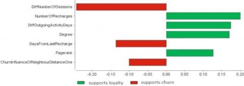
The attribute importance of the developed GBT model is shown in Figure 5. Red bars show that these attributes DiffNumber of Sessions, Days from Last Recharge and Churn Influence of Neighbour Distance One support a higher probability of user churn. Green bars show that the attributes Number of Recharges, DiffOutgoing Activity Days, Degree and Pagerank support loyal telecom users.
Figure 5. Attribute importance of developed models
From Figure 5 we can see that the two most important attributes for predicting telecom churn are behavioural attributes DiffNumber of Sessions and Number of Recharges. Nevertheless, SNA attributes Churn Influence of Neighbour Distance One, Degree and Pagerank are also very important to use for predicting telecom churn. We can see that the newly developed measure Churn Influence of Neighbour Distance One is a valuable attribute that indicates the churn propensity of a telco user. This also shows us that directly connected users have a greater influence on the propensity of telco churn than indirectly connected users.
This paper presents a brief overview of the research in the topics of telecom churn prediction, Social Network Analysis and AutoML. In our research, for creating telecom churn prediction models, we proposed and used an upgraded AutoML model with the SNA addition. In our work, we define and develop two new social attributes Churn Influence of Neighbour Distance One and Churn Influence of Neighbour Distance Two that measure the social influence of already churned users. Our experiment shows that it is valuable to use these new measures and that directly connected users have a greater influence on the propensity of telco churn than indirectly connected users. We developed two models that use SNA measures and two models without SNA measures and compare them. Developed models with SNA attributes have higher measure values than models developed without SNA attributes. Therefore, we can conclude that it is useful to create SNA measures to obtain greater accuracy of the model.
An experiment in this work was made with AutoML, and it is shown that good results can be obtained using the AutoML and SNA attributes. Comparison of developed models shows us that the GBT algorithm has a better result than the deep learning algorithm and we can conclude that the best-developed model is the GBT with SNA attributes. Based on the GBT churn prediction model with SNA attributes telecom companies can build various marketing approaches to retain potential churners. The value of the model from this paper is further reflected in the fact that using AutoML it is possible to develop new models very fast. Fast model development allows telecom companies to easily adapt to changes in the dynamic telecom market. Since the churn prediction models are highly dependent on the data, future research could use other data sets to verify the findings from this work.
[1] Hassouna, M., Tarhini, A., Elyas, T., AbouTrab, M.S. (2015). Customer churn in mobile markets: A comparison of techniques. International Business Research, 8: 224-237. https://doi.org/10.5539/ibr.v8n6p224
[2] Lazarov, V., Capota, M. (2007). Churn prediction. Business Analytics Course. TUM Computer Science.
[3] Joshi, S. (2014). Customer experience management: An exploratory study on the parameters affecting customer experience for cellular mobile services of a telecom company. Procedia - Social and Behavioral Sciences, 133: 392-399. http://doi.org/10.1016/j.sbspro.2014.04.206
[4] Amin, A., Anwar, S., Adnan, A., Nawaz, M., Howard, N., Qadir, J., Hawalah, A., Hussain, A. (2016). Comparing oversampling techniques to handle the class imbalance problem: A customer churn prediction case study. IEEE Access, 4: 7940-7957. http://doi.org/10.1109/ACCESS.2016.2619719
[5] Mozer, M.C., Wolniewicz, R., Grimes, D.B., Johnson, E., Kaushansky, K. (2000). Predicting subscriber dissatisfaction and improving retention in the wireless telecommunications industry. IEEE Trans Neural Networks, 11(3): 690-696. http://doi.org/10.1109/72.846740
[6] Umayaparvathi, V., Iyakutti, K. (2012). Applications of data mining techniques in telecom churn prediction. International Journal of Computer Application, 42(20): 5-9. http://doi.org/10.5120/5814-8122
[7] Umayaparvathi, V., Iyakutti, K. (2016). Attribute selection and customer churn prediction in telecom industry. International Conference on Data Mining and Advanced Computing, pp. 84-90. http://doi.org/10.1109/SAPIENCE.2016.7684171
[8] Ahmad, A.K., Jafar, A., Aljoumaa, K. (2019). Customer churn prediction in telecom using machine learning in big data platform. Journal of Big Data, 6: 28. http://doi.org/10.1186/s40537-019-0191-6
[9] Ullah, I., Raza, B., Malik, A.K., Islam, S.U.L., Kim, S.W., Imran, M. (2019). A churn prediction model using random forest: Analysis of machine learning techniques for churn prediction and factor identification in telecom sector. IEEE Access, 7: 60134-60149. http://doi.org/10.1109/ACCESS.2019.2914999
[10] Mandić, M., Kraljević, G. (2020). Two-layer architecture of telco churn Auto-ML. Proceedings of the 31st International DAAAM Symposium, 31: 788-792. http://doi.org/10.2507/31st.daaam.proceedings.109
[11] Brandusoiu, I., Toderean, G., Beleiu, H. (2016). Methods for churn prediction in the pre-paid mobile telecommunications industry. 2016 International Conference on Communications, pp. 97-100. http://doi.org/10.1109/ICComm.2016.7528311
[12] Idris, A., Khan, A. (2017). Churn prediction system for telecom using filter-Wrapper and ensemble classification. The Computer Journal, 60: 410-430. http://doi.org/10.1093/comjnl/bxv123
[13] Castanedo, F., Valverde, G., Zaratiegui, J., Vazquez, A. (2014). Using deep learning to predict customer churn in a mobile telecommunication network. 1-8.
[14] Umayaparvathi, V., Iyakutti, K. (2017). Automated feature selection and churn prediction using deep learning models. International Research Journal of Engineering and Technology, 4(3): 1846-1854.
[15] Mandić, M., Davor, Š., Martinović, G. (2018). Clique comparison and homophily detection in telecom social networks. International Journal of Electrical and Computer Engineering Systems, 9: 81-87. http://doi.org/10.32985/ijeces.9.2.5
[16] Ouyang, Y., Hu, M.M., Huet, A., Sun, X. (2016). Mining of leaders in mobile telecom social networks. Wireless Telecommunications Symposium, pp. 4-7. http://doi.org/10.1109/WTS.2016.7482054
[17] Varun, E., Ravikumar, P. (2016). Telecommunication community detection by decomposing network into n-cliques. International Conference on Emerging Technological Trends, pp. 1-5. http://doi.org/10.1109/ICETT.2016.7873770
[18] Chang, Y.C., Lai, K.T., Chou, S.C., Chen, M.S. (2017). Mining the networks of telecommunication fraud groups using social network analysis. Proceedings of the 2017 IEEE/ACM International Conference on Advances in Social Networks Analysis and Mining, pp. 1128-1131. http://doi.org/10.1145/3110025.3119396
[19] Oliveira, M., Gama, J. (2012). An overview of social network analysis. WIREs Data Mining and Knowledge Discovery, 2: 99-115. http://doi.org/10.1002/widm.1048
[20] Pushpa, S. (2021). An efficient method of building the telecom social network for churn prediction. International Journal of Data Mining & Knowledge Management Process, 2: 31-39. http://doi.org/10.5121/ijdkp.2012.2304
[21] Gamulin, N., Štular, M., Tomazic, S. (2015). Impact of social network to churn in mobile network. Automatika, 56: 252-261. http://doi.org/10.7305/automatika.2015.12.742
[22] Kostić, S.M., Simić, M.I., Kostić, M.V. (2020). Social network analysis and churn prediction in telecommunications using graph theory. Entropy, 22: 1-23. http://doi.org/10.3390/e22070753
[23] Nagarajah, T., Guhanathan, P.A. (2019). Review on automated machine learning (AutoML) systems. IEEE 5th International Conference for Convergence in Technology, pp. 1-6. http://doi.org/10.1109/I2CT45611.2019.9033810
[24] Chapman, P., Clinton, J., Kerber R., et al. (2000). Crisp-Dm 1.0. Step-by-step data mining guide. SPSS. 76.
[25] Thornton, C., Hutter, F., Hoos, H.H., Leyton-Brown, K. (2013). Auto-WEKA: Combined selection and hyperparameter optimization of classification algorithms. In Proceedings of the 19th ACM SIGKDD International Conference on Knowledge Discovery and Data Mining, pp. 847-855. http://doi.org/10.1145/2487575.2487629
[26] Hutter F., Kotthoff L., Vanschoren J. (2019). Automated machine learning. The Springer Series on Challenges in Machine Learning, 39-68. http://doi.org/10.1007/978-3-030-05318-5_2
[27] Ferreira, L., Pilastri, A., Martins, C., Santos, P., Cortez, P. (2020). An automated and distributed machine learning framework for telecommunications risk management. Proceedings of the 12th International Conference on Agents and Artificial Intelligence, 2: 99-107. http://doi.org/10.5220/0008952800990107
[28] Zhao, M., Zeng, Q., Chang, M., Tong, Q., Su, J. (2021). A prediction model of customer churn considering customer value: An empirical research of telecom industry in China. Discrete Dynamics in Nature and Society, pp. 1-12. http://doi.org/10.1155/2021/7160527
[29] Gong, F., Ma, Y., Gong, W., Li, X., Li, C., Yuan, X. (2018). Neo4j graph database realizes efficient storage performance of oilfield ontology. PLoS One, 13: 1-16. http://doi.org/10.1371/journal.pone.0207595
[30] Pokorný, J. (2015). Graph databases: Their power and limitations. Computer Information Systems and Industrial Management, 9339: 58-69. http://doi.org/10.1007/978-3-319-24369-6_5
[31] Wasserman, S., Faust, K. (1994). Social network analysis: Methods and applications. Cambridge University Press, http://doi.org/10.1017/CBO9780511815478
[32] Beauchamp, M.A. (1965). An improved index of centrality. Behavioral Science, 10(2): 161-163. http://doi.org/10.1002/bs.3830100205
[33] Bihari, A., Pandia, M. (2015). Eigenvector centrality and its application in research professionals’ relationship network. 1st International Conference on Futuristic Trends in Computational Analysis and Knowledge Management (ABLAZE), pp. 510-514. http://doi.org/10.1109/ABLAZE.2015.7154915
[34] Li, J., Willett, P. (2009). ArticleRank: A PageRank-based alternative to numbers of citations for analysing citation networks. Aslib Proceedings, 61: 605-618. http://doi.org/10.1108/00012530911005544