Le Quang Thao* | Duong Duc Cuong | Nguyen Tuan Anh | Nguyen Minh | Nguyen Duc Tam
© 2022 IIETA. This article is published by IIETA and is licensed under the CC BY 4.0 license (http://creativecommons.org/licenses/by/4.0/).
OPEN ACCESS
Greenhouses are considered to be a favorable artificial environment separated from the outside. However, pests can still exist by the same plant sources that bring the pathogen. The conditions and abundant food in a greenhouse provide a stable environment for the pest development. Normally, the natural enemies that serve to keep pests under control outside are not present in the greenhouse, pest situations often develop in this indoor environment more rapidly and with greater severity than outdoors. Early detection and diagnosis of pests and diseases are key to managing greenhouse pests as well as selecting and applying appropriate pesticides when needed. The aim of this invention is to develop an intelligent pest early detection system using a convolutional neural network in the greenhouse. By using a pre-trained disease recognition model, we were able to perform deep transfer learning to produce a network that can predict with the precision above 90%.
pests, greenhouse, transfer learning, SSD Lite MobileNet V2
Agriculture plays an important role in our daily lives because it provides food for daily consumption and for social needs. Agriculture is a primary production sector and plays a major role in fighting poverty for developing countries [1]. In addition to factors such as soil, nutrition, water, minerals that affect crop quality, pests and diseases are also considered as one of the main factors affecting plant development and productivity [2]. Numerous studies have shown that pests and diseases greatly affect crops [3]. According to the National Geographic report, grasshoppers in Africa, the Middle East and Asia can destroy 423 million pounds of crops every day, causing losses of about 82 million US dollars [4]. Another example is fungus related diseases, which affect many plants, caused by a variety of fungi species. It usually produces a powdery mildew substance that grows on both sides of the leaf. These leaves can be twisted, deformed, then wilted and died from the infection, or as some other fungal disease reduces the photosynthesis process takes place, prevents respiration and evaporation, and causes the growth slower. To overcome pests and diseases that affect crop yields, one of the solutions used is the greenhouse [5]. Greenhouse is a model in which plants can grow and develop with the best conditions for each specific species, while also helping minimize the risks that nature brings to plants. It can bring a very high economic efficiency than the form of outdoor farming [6]. However, pests and diseases can still exist in the greenhouses from varying sources:
(1) Eggs, nymphs of many harmful insects; spores of various diseases lurking in the soil, in the bushes, grasses, etc.
(2) Using seeds and seedlings infected with insects and diseases causes pests and diseases to exist.
For that reason, early detection of pests and diseases in greenhouses is the most important key point to crop management. It prevents damage and loss, thus increasing production and significantly contributes to a nation’s food security. There are many existing methods for crop management such as locating the geological location of pests and their natural enemies, for example, spiders were used against rice pests to protect the crop in Korea [7]. This method is eco-friendly, but other problems may appear when applied in a greenhouse environment. Another way is using devices such as traps to capture fruit flies in tarweed plants [8]. This technique shows efficiency with a large area, but if this was used in the greenhouse, the area of the traps will affect the distribution of lights in the greenhouse. Another simple but troublesome solution is using pesticides. However, these substances release many toxic elements to the environment, and governments usually have a very restricted list of allowed substances and amounts.
With the rising of computer vision and Artificial Intelligence (AI), Selvaraj et al. applied AI with transfer learning to detect banana diseases to create banana mobile app management [9] or Türkoğlu and Hanbay using deep learning-based features to detect plant diseases and pests to provide automatic diagnosis of plant diseases with visual inspection [10].
In order to use in reality and be able to use on mobile embedded systems such as Raspberry Pi, we apply a transfer learning method using Single Shot Multibox detector Lite [11] (SSD Lite) architecture with MobileNetV2 [12] model to train pest images obtained from the greenhouse. This is executed on the server, and the result after training will be transferred to a single board computer (SBC) to detect and classify pests. We believe that our project will improve food quality and quantity, prevent plant’s diseases, chemical substances and reduce human health risks.
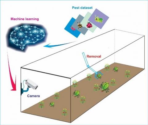
2.1 System block diagram
In our greenhouse we have two parts as shown in Figure 1. The first to train the machine learning model on the server. We use only 3 common types of pests in the greenhouse to prepare the dataset for training such as Cabbage looper, Colorado potato beetle and Cutworm. These images were taken under various conditions such as different light conditions, focal lengths and rotating positions, and resized to 300 x 300 pixels for training with the SSD Lite MobileNetV2 pre-trained model.
The second is recognition in the greenhouse, which is a Raspberry Pi SBC with configuration shown as in Table 1 and a fixed camera to provide a video stream of the pest. The camera is installed on top of the greenhouse to observe the crop below. Since pests are constantly moving around, when we use a camera with sufficiently high resolution, there will probably be no blind spot in most cases. In case the greenhouse area is too large, the camera does not have high enough resolution, or there exists a blind spot on the farm plot, we will consider moving both Raspberry Pi and the camera mounted to the drone, or moving along the axis of the greenhouse It will detect and classify pests from the obtained video based on training results from the server in the first part. The result will be sent to the central monitor to help users control pests in the real-time by removing or applying appropriate pesticides when needed.
Figure 1. Diagram of the main block system
Table 1. Raspberry Pi configuration
|
|
Specifications |
|
CPU |
ARM Cortex A53 of 1.2 GHz |
|
GPU |
400 MHz VideoCore IV multimedia |
|
Memory |
1GB LPDDR2 |
|
GPIO |
17 GPIO plus specific functions |
|
Connectivity |
Ethernet, Wlan, Bluetooth |
|
Software |
Python, OpenCV-library |
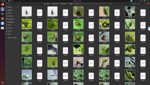
Our dataset consists of 200 photos taken in the greenhouse as mentioned above, of which 120 are used for training and 80 are used for testing. After taking pictures of common pests in the greenhouse, we preprocessed the images, resizing them into 300x300 pixels but still keeping the images of pests, the distribution of each pest type as shown in Table 2. Training photos are needed for the model to learn the features of pests, and testing photos are needed to evaluate the performance of the model. After collecting the data, we will have to label the images. The process of labeling images is done by LabelImg software [13].
Table 2. Distribution of pest dataset
|
|
Training |
Testing |
|
Cabbage looper |
38 |
24 |
|
Colorado potato beetle |
43 |
29 |
|
Cutworm |
39 |
27 |
|
Total |
120 |
80 |
2.3 Transfer learning and CNN architectures
2.3.1 Transfer learning
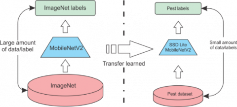
Transfer learning [14] is a popular method in computer vision because it allows us to build an accurate model without wasting time. The idea of transfer learning is very simple. Instead of the traditional machine learning method, which is used for each task, we create a model to solve only that problem. Transfer learning uses the knowledge gained from solving a previous problem and applies that knowledge to a different but related problem. In computer vision, transfer learning is often shown through the use of pre-trained models (for example: VGG, Inception, MobileNet). A pre-trained model is a model that has been trained on a big dataset to solve a related problem to the problem that we want to solve. Transfer learning helps to save time and dramatically reduce the amount of data and labels needed to train for the current model because it has applied knowledge learned from previous models into the current model. This process is shown as in Figure 2.
For pest early detection, we train the model using SSD Lite architecture with the pre-trained MobileNetV2 model. Which was trained on the ImageNet dataset with one million images. Currently, ImageNet is one of the well-labeled datasets for learning general-purpose tasks. By using the pre-trained model from the beginning to recognize the features of the image like shape, color of pests, it will be more convenient to re-train on our labeled pest dataset.
Figure 2. Basic flow of transfer learning
2.3.2 SSD Lite MobileNetV2 model
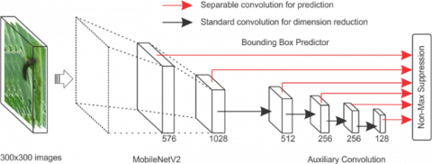
The architecture of SSD Lite [11] is that the regular convolutions are replaced by depth wise separable convolutions in the predictive layers and the whole process is done in a single phase. SSD Lite extracts feature maps and applies convolution filters in Conv4_3 class to detect, classify and accurately identify object containers. In SSD Lite, multibox is a technique that uses multiple bounding boxes suitable for all objects, large and small, including pests and diseases for this project. The Non-Maximum Suppression (NMS) at the end of the architecture is used to retain only the best predictions of the model by setting the threshold to preserve highly overlapping objects and predict very small bounding boxes that are compact for all cases. By changing the threshold value, we realized that if the value is too low, then it will increase the chance of overlapping the predictions. However, if the value is too big, it’ll be very difficult to differentiate entities that are close to another one. After performing the threshold, we picked a fixed and suitable value of NMS = 0.45 to balance our predictions.
MobileNetV2 pre-trained model is a model used to classify objects for mobile devices proposed [12]. This model uses linear bottleneck and inverted residuals for improving performance. The bottleneck takes in compressed low performance and expands, improves it into high performance, and then turns back into compressed low performance by applying depth-wise separable convolutions into the bottleneck, and using a linear convolution. This process reduces the chance of information loss and saves memory more than the original bottleneck. It improves the performance of mobile models on multiple tasks and benchmarks as well as on the spectrum of different model sizes with some advance feature:
Bottlenecks encode average inputs and outputs, while the inner layer encapsulates the ability to convert from low-level concepts like pixels to higher levels like the model categories of the model Finally, with other traditional residual connections, shortcuts allow for faster training with greater accuracy. When SSD Lite was applied to MobileNetV2, the number of parameters and the computational cost were significantly reduced. Moreover, it can be used on a low power-consumption SBC such as a Raspberry Pi B. SSD Lite replaces all the regular convolutions with separable convolutions in the SSD predict layer, thereby helping to significantly reduce the parameters and computational costs. The sub-network stack of SSD Lite is based on auxiliary convolutional feature layers, which are designed such that they decrease in size in a progressive manner, thus enabling the flexibility of detecting objects within a scene across different scales. The SSD Lite MobileNetV2 model that we used has the following structure as shown in Figure 3.
Figure 3. SSD lite MobileNet V2 model
2.3.3 The algorithm for transfer training
The following steps summarize SSD Lite MobileNetV2:
3.1 Pest dataset collection and labeling
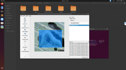
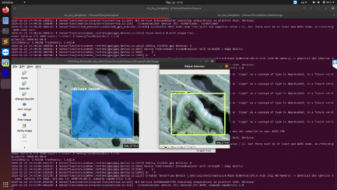
We use the software LabelImg on Ubuntu operating system to label the images, then create a separate conda environment for LabelImg. After that, when labeling is shown as in Figure 4, the type of class and coordinates of the boxes are saved as “xml” files shown as in Figure 5.
Each label represents a different type of pests. Each image may contain more than one label depending on the number of infected areas of the crop. The LabelImg file is saved as a “pbtxt” and later converted to “TFrecord” format. Finally, we split our dataset into 2 subsets, training and testing, for training on the server.
After training, some types of pests are noticed for high accuracy up to 99% as shown in Figure 6. However, if the pest is curved to the abnormal shape or size of the pest, the system will fail to recognize the insect. We also observed that during the labeling process, a single class for an image worked as a ground-truth bounding box for the model.
Figure 4. Labeling images
Figure 5. Dataset and xml file
Figure 6. Comparison between labeling and result
3.2 Training process
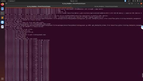
After all images are extracted to "TFrecord", we perform transfer learning with the feature server in Table 3. The time for training images lasts for 15 hours 21 minutes and the training process is shown as in Figure 7.
Table 3. Server to train
|
|
Values |
|
CPU |
Intel® X3450@2.67 GHz x 8 |
|
GPU |
GeForce GTX 750 Ti/PCle/SSE2 |
|
Memory |
RAM 16Gb, HDD 256Gb |
|
OS |
Ubuntu 18.04.3 LTS |
|
Program |
LabelImg, Python, OpenCV library |
|
bash_size |
8 |
|
num_class |
5 |
Figure 7. Training process
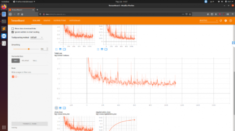
3.3 Loss function
Loss function is a value that shows the error between the training data and the testing data. In our project, we considered two losses which are localization loss ($L_{l o c}$) and confidence loss ($L_{\text {conf }}$). Total loss is a weighted sum of the $L_{l o c}$ and the $L_{\text {conf }}$ given in the following equation:
$L_{(x, c, l, g)}=\frac{1}{N}\left(L_{\text {conf }}(x, c)+\alpha L_{l o c}(x, l, g)\right)$ (1)
where, $L_{l o c}$ is the localization loss which is the smooth $L_{1}$ loss between the predicted box $(l)$ and the ground-truth box $(g)$ parameters. These parameters include the offsets for the center point $(c x, c y)$, width $(w)$ and height $(h)$ of the bounding box expressed as the following equation:
$L_{l o c}(x, l, g)=\sum_{i \in P o s}^{N} \sum_{m \in\{c x, c y, w, h\}} \quad x_{i j}^{k} \operatorname{smooth}_{L 1}\left(l_{i}^{m}-\hat{g}_{j}^{m}\right)$ (2)
Figure 8. Loss function graph
$L_{\text {conf }}$ is the confidence loss which is the softmax loss over multiple classes of confidences $(c), \alpha$ is set to 1 by cross validation, $x_{i j}^{p}=[1,0]$ is an indicator for matching $i-t h$ default box to the $j-t h$ ground truth box of category $p$ represented by the following equation:
$L_{\text {conf }}(x, c)=-\sum_{i \in P o s}^{N} x_{i j}^{p} \log \left(\hat{c}_{i}^{p}\right)-\sum_{i \in P o s} \log \left(\hat{c}_{i}^{0}\right)$ (3)
The value of the loss function is directly corresponding to the model performance as shown in Figure 8.
At first, the model can only perform minor detection such as line detection, shape detection, etc. Therefore, the model when compared with the testing dataset creates a high loss value. After later iterations, the model can combine minor detection to form object detection. This is when the loss value decreases dramatically. The training process will stop when the loss value is smaller than 0.8 and the other near value remains constant for a long time.
3.4 Metric evaluation
Although accuracy rate is one of the most representative values to use when evaluating the model, to calculate that we certainly need to base it on 4 fundamental values in prediction evaluation: True Positive (TP), True Negative (TN), False Positive (FP) and False Negative (FN). In comparison to the ground truth, we have:
True Positive: 37, is the number of samples that the model predicted to be in one class, and in fact belong to that class.
False Positive: 2, is the number of samples that the model predicted to be in one class, but in fact do not belong to that class.
True Negative: 40, is the number of samples that the model predicted NOT to be in one class, and in fact do not belong to that class.
False Negative: 1, is the number of sample(s) that the model predicted NOT to be in one class, but in fact belong to that class.
With these 4 pillar values, we can now calculate the scores to evaluate the model. There are several formulas representing different aspects of the model, but here we just list some most commonly used:
Sensitivity, as known as (AKA) Recall or True Positive Rate (TPR) is the probability of a positive prediction being true:
$T P R=\frac{T P}{T P+F N}=\frac{37}{37+1} \approx 97 \%$ (4)
Specificity, AKA Selectivity or True Negative Rate (TNR) is the probability of a negative prediction being true:
$T N R=\frac{T N}{T N+F P}=\frac{40}{40+2} \approx 95 \%$ (5)
As we can see, these two values when calculated alone do not represent the performance of the model, since it only needs to predict everything as positive or negative to get a 100% on TPR or TNR. Thus, we need other values in order to be able to evaluate the true performance of the model, such as:
Precision or Positive Predictive Value (PPV) is the rate of correct positive predictions over all positive predictions, representing the performance of the model when it comes to positive tests:
$P P V=\frac{T P}{T P+F P}=\frac{37}{37+2} \approx 95 \%$ (6)
Negative Predictive Value (NPV) is the rate of correct negative predictions over all negative predictions, representing the performance of the model when it comes to negative tests:
$N P V=\frac{T N}{T N+F N}=\frac{40}{40+1} \approx 98 \%$ (7)
Accuracy (ACC) represents the performance of the model when it comes to both positive and negative tests, with a relatively simple equation:
$A C C=\frac{T P+T N}{T P+T N+F P+F N}=\frac{37+40}{37+40+20+1} \approx 96 \%$ (8)
F1-score: Another value representing the model’s performance overall, based on the harmonic mean of Sensitivity and Precision:
$F 1=2 \times \frac{P P V \times T P R}{P P V+T P R}=2 \times \frac{0.97 \times 0.95}{0.97+0.95} \approx 96 \%$ (9)
3.5 Pest detection on the mobile device
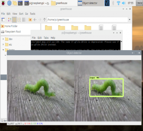
In this project, we labeled all images, trained the model using transfer learning on the server, and produced an inference graph. After testing, we noticed that the model can detect pests in real-time as shown in Figure 9.
Figure 9. Correct detection
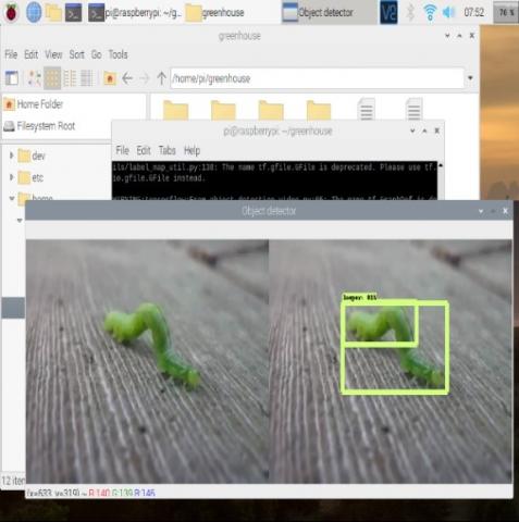
Figure 10. Incorrect detection
Figure 11. A prototype of the system
However, some detections are incorrect due to abnormal shapes or colors, such as overlapping bounding boxes as shown in Figure 10. Because our dataset only contains 200 training and testing images, therefore, in the multibox layer, the model cannot detect the insect, which causes overlapping bounding boxes.
3.6 Prototype of system
After designing and investigating, our group finished the system. The final prototype of our project is shown as in Figure 11.
In our prototype of the system, we created a model with trees and some types of pests. It included a camera attached to a Raspberry Pi SBC to collect the pests' images in the greenhouse for the detection. Here are the models of the pests which were artificially provided but not the natural pests. During the test, we changed the pests in many positions, and the accurate prediction output was up to 96% under laboratory conditions.
In this work, we applied transfer learning based on SSD Lite architecture using MobileNetV2 as the backbone for the pest classifying application. While the inference time is still not desirable as the camera configuration has not reached 1080p@30fps, the model’s accuracy is already high enough to be used in real life condition if we reduce the camera’s FPS. We believe our model can be furthermore improved with a larger dataset for training and testing, although we still make our self-collected dataset available for the public. Some work planned to be done in the future are:
[1] Johnston, B.F., Mellor, J.W. (1961). The role of agriculture in economic development. The American Economic Review, 51(4): 566-593.
[2] Headey, D., Alauddin, M., Rao, D.P. (2010). Explaining agricultural productivity growth: An international perspective. Agricultural Economics, 41(1): 1-14. https://doi.org/10.1111/j.1574-0862.2009.00420.x
[3] Dhanush, D., Bett, B.K., Boone, R.B., et al. (2015). Impact of climate change on African agriculture: Focus on pests and diseases. CCAFS Info Note. Copenhagen, Denmark: CGIAR Research Program on Climate Change, Agriculture and Food Security (CCAFS).
[4] National Geographic Information, www.nationalgeographic.com.
[5] Teitel, M., Montero, J.I., Baeza, E.J. (2011). Greenhouse design: Concepts and trends. In International Symposium on Advanced Technologies and Management Towards Sustainable Greenhouse Ecosystems: Greensys2011, Athens, Greece, pp. 605-620. http://dx.doi.org/10.17660/ActaHortic.2012.952.77
[6] Growcer Robotic Urban Farming, www.growcer.com.
[7] Lee, J.H., Kim, S.T. (2001). Use of spiders as natural enemies to control rice pests in Korea (Vol. 501). Food and Fertilizer Technology Center.
[8] Krimmel, B.A., Pearse, I.S. (2013). Sticky plant traps insects to enhance indirect defence. Ecology Letters, 16(2): 219-224. https://doi.org/10.1111/ele.12032
[9] Selvaraj, M.G., Vergara, A., Ruiz, H., Safari, N., Elayabalan, S., Ocimati, W., Blomme, G. (2019). AI-powered banana diseases and pest detection. Plant Methods, 15(1): 92. https://doi.org/10.1186/s13007-019-0475-z
[10] Türkoğlu, M., Hanbay, D. (2019). Plant disease and pest detection using deep learning-based features. Turkish Journal of Electrical Engineering & Computer Sciences, 27(3): 1636-1651. http://dx.doi.org/10.3906/elk-1809-181
[11] Liu, W., Anguelov, D., Erhan, D., et al. (2016). SSD: Single shot multibox detector. Computer Vision – ECCV 2016, Amsterdam, the Netherlands, pp. 21-37. https://doi.org/10.1007/978-3-319-46448-0_2
[12] Sandler, M., Howard, A., Zhu, M., Zhmoginov, A., Chen, L.C. (2018). Mobilenetv2: Inverted residuals and linear bottlenecks. In Proceedings of the IEEE Conference on Computer Vision and Pattern Recognition, Lake City, UT, USA, pp. 4510-4520. https://doi.org/10.1109/CVPR.2018.00474
[13] LabelImg Soft, https://github.com//tzutalin/labelImg.
[14] Torrey, L., Shavlik, J., (2009). Transfer Learning. Handbook of Research on Machine Learning Applications. https://ftp.cs.wisc.edu/machine-learning/shavlik-group/torrey.handbook09.pdf.