Zahira Chouiref* | Mohamed Yassine Hayi
© 2022 IIETA. This article is published by IIETA and is licensed under the CC BY 4.0 license (http://creativecommons.org/licenses/by/4.0/).
OPEN ACCESS
With the development of machine learning, to improve the accuracy in recommendation systems, the main purpose of the suggested approach consists of using techniques and algorithms which can predict and suggest relevant tourist services (k-items) to users according to their interests, needs, or tastes. In this research, we describe how machine learning techniques can automatically provide personalized recommendations to the requestors by considering both their preferences and their implicit/explicit contextual information and the current contextual constraints of the points of interest. We build an efficient, intelligent H-RN algorithm that hybridizes both the most known machine learning algorithms, namely Random Forest and Naïve Bayes, with both collaborative filtering techniques (model-based and memory-based technique). Different experiments of our approach as part of a recommender system in the touristic field are performed over the four large real-world datasets. Recommender systems can use H-RN to improve recommendation prediction and reduce the search space of tourist services. Moreover, the results of recall, precision, accuracy, F-measure, and average rate, as well as a set of statistical tests (One-way ANOVA, Diversity) and error metrics (RMSE, MAE) have been discussed to show the improvement of the prediction accuracy of our algorithm compared to the baseline approaches in various settings.
context-awareness, machine learning, Random Forest, Naïve Bayes, Neural Network, K-Nearest Neighbor recommendation, tourist services
The explosive growth of services over the Internet and the diversity of user preferences have conducted to a difficulty in selecting the best services that meet the user's needs in terms of preferences and context. Moreover, the service requestors are often faced with many competing services that offer “similar” functionalities. However, they are associated with “different” contextual constraints and they need to select the best ones from the list of items with required functionalities and the highest desired quality. We are frequently exposed to situations that lead us to make decisions and make choices, such as movies, music, scientific articles, products, places of vacation, etc. The recommendation consists of selecting relevant suggestions based on the choices which users make. Recommender Systems (RSs) have been developed to anticipate user needs, offer them relevant items in a vast space of resources according to their preferences, and make an accurate prediction of whether a given user will like an item [1]. The RS evolved to actively recommend the right items to online users, typically without an explicit search query. To achieve such a goal and provide personalized recommendations, an RS needs to accumulate data on users and/or available items, i.e., the RS must know the preferences of each user before applying computational intelligence techniques [2] (statistical or bio-inspired computing techniques) to predict the best items. The personalized recommendation systems have been implemented in many real-life applications and business domains. They have proven to be successful in movie and music, social networks, healthcare, personalized news, etc., but appear to be limited in tourism. Today, tourism is of great importance to the worldwide economy, and it involves the propagation of large amounts of information [3]. In the field of tourism, the recommendation can be made in various situations such as personalized route recommendation [4], smart itinerary recommendation like proposed in our previous work [5], Point of Interest (POIs) recommendation [6, 7], etc. In the last decade, several approaches for RSs have been proposed to cope with these challenges. Unfortunately, current RSs (e.g., tourism service recommender systems) are rigid as they are completely isolated from various concepts of user “preferences” and/or “context”. For instance, such rigidness results in non-suitable services (e.g., a visitor may get mountain tourism with a very bad climate instead of visiting to the museum in these bad weather conditions). Some important aspects should be considered to improve the recommendation process, like the context of a tourist destination visited, weather forecast, etc.
Machine learning (ML) is a field that tries to make computers learn patterns without explicit programming [2]. The rapid advance of ML has enabled a new paradigm of con-text-awareness in RSs, so this paradigm is an ML for context-aware recommender systems. This research proposes a new recommendation method based on ML algorithms to enhance the predictive accuracy of RSs in the tourism domain. Indeed, a tourism personalized recommendation system should involve the following characteristics:
(1) It should extract user's preferences and interests by using both historical and current data,
(2) It should leverage part of the characteristics of the user and the contextual constraints of recommendation object to foresight the future and improve the matching process,
(3) It should also contribute context-aware recommendations, which are already adapted to the user’s current situation.
Motivated by the issues mentioned above, in sharp contrast to the existing approaches that focus only on user-specified information, in this paper, we propose an effective approach, which gives users an adequate way in order to take into account their explicit/implicit preferences and enhance the service recommendation by leveraging their contexts extracted at real-time. In our case study, RS allows to adapt and personalize the user's visit according to a context, taking into account their preferences and constraints. The tourist selects what he considers his POIs, but some contextual aspects need to be considered to make a context-aware recommendation. Accordingly, to make an intelligent context-aware recommendation, this research proposes a hybrid recommendation approach made up of both memory-based and model-based Collaborative Filtering (CF). CF-based tourism recommender system finds those users that, although they do not have a direct relationship with the tourist service, still look like other users who have such relationships. In such a system, a user readily reveals his preferences over items to the system, intending to obtain valuable recommendations. We use explicit preferences, nevertheless, some attributes stay implicit. The proposed system learns something about the context of a tourist service to recommend the best destinations to the specific tourist. For example, consider the case where a user is interested in mountain tourism. If the climate is very bad, a tourist may not get mountain tourism, so a smart tourist system must recommend in real-time a visit to the museum in these bad weather conditions. For this reason, taking into account the implicit information to recommend the best one is an important point. The proposed CF recommender tends to improve the accuracy as the amount of data over items grows. The CF algorithm predicts customers’ preferences by calculating similarities among customers or items [8].
The recommender system is tested on the four most used machine learning algorithms, in particular Neural Network (NN), K-Nearest Neighbor (KNN), Naïve Bayes (NB), and Random Forest (RF). The proposed system additionally applies the hybridization of the last two algorithms. This hybridization allows to extracts and utilizes the information relative to context about each candidate tourist services in real-time and leverage the contextual constraints related to the user's location (in order to identify the POI around him/her) and weather conditions of the user visit (to provide more relevant recommendations that are appropriate to the current weather situation). However, up to now, none of the existing tourism recommendation systems have studied the above hybridization. Hence, the proposed context-aware tourism recommendation algorithm which is based on ML techniques, is applied to extracted data from four real-world datasets namely (i) TripAdvisior, (ii) Dataset_tsmc, (iii) Hotel_Reviews, and (iv) dataset_ubicomp to make comparisons between the efficiency of the different recommendation algorithms and to evaluate the proposed system. The evaluation criteria (recall, precision, F-measure, accuracy, average rate), the statistical tests (One-way ANOVA, Diversity), and the error metrics (RMSE, MAE) in this work show that our proposal can improve existing algorithms, which is depicted in results analysis subsection. In addition, performance assessments via extensive simulations are conducted, and the results also demonstrate their effectiveness and efficiency for reliable service selection in tourism applications. The proposed approach was developed using Python. Therefore, the remainder of this paper is organized as follows: Section 2 briefly reviews the related literature on context-awareness and machine learning in RS. Section 3 highlights our hybrid recommendation approach. Section 4 describes results analysis and performance evaluation, followed by the conclusion and future works in Section 5.
This research deals with a tourism recommendation system that extracts users’ preferences and uses contextual information to provide personalized recommendations. This section briefly reviews some related work that target context-awareness and machine learning techniques in RS.
2.1 Context-aware recommendation systems
The recommender systems, also called the information filtering systems, allow to suggest only the information which interests the user, and it eliminates the information that is not relevant. The purpose of RS is to model user tastes (preferences) in order to suggest (recommend) invisible content that users would find interesting [4]. Thus, the two essential tasks of RS are:
(1) Predicting user opinion (e.g., rating) on a set of items.
(2) Predicting and recommending a set of correct (interesting, useful) items for the user.
Several types of research have been done on context-aware recommendation field: Social Aware Recommender System [9], prediction systems [10] where the authors predict the next place based on one trajectory dataset but with systematically varying prediction algorithms, methods for space discretization, scales of prediction (based on a novel hierarchical approach), and incorporated context data. The context represents the environment in which the visitor operates. In our case, it depends on the weather data and the distance to the POI where in both cases, we distinguish two types of actions: voluntary action such as the user's position, or involuntary action like weather conditions (if a parameter of the weather state were to change or the weather conditions become unfavorable). So, the problem we are asking in this paper is whether the change in the environment affects the items to recommend.
The current location is the most important element used in general tourism recommendation systems [11, 12]. Recently, there has been extensive research on studying context-aware recommender systems in tourist services. These researches have highlighted several investigations, such as Ref. [13], that propose the location-context-awareness recommendation system using the hierarchical model, which is based on long-short-term memory (LSTM) (Long-Short Term Memory). This model predicts the probability of a user's next visit to a tourist site and then incorporates contextual data to recommend the best places to the user. The proposed LSTM model works better on the dataset than the Naïve Bayes machine learning model, the Markov model such as WMM and the other deep learning models such as GRU or two-way LSTM. This work [14] proposes a context-aware recommender system named CAT-TOURS that uses temporal ontology and the NB algorithm. It allows finding a simple method to categorize Thailand tourism web documents containing information on more than one topic and take time constraints into account in formulating recommendations. That work recommended tourist information depending on time and season by applying the temporal ontology.
According to Ref. [15], RecUFG is a personalized tourist attraction recommendation algorithm that combines the technology of collaborative user filtering with the relationships of trust between friends and the geographical context to solve the problem of the weak precision of the personalized tourist recommendation system. In this study, the main data source is the user location information (LBSN) and the Flickr site. Experimental results on real data sets demonstrate the feasibility and efficiency of the algorithm compared to the existing recommendation algorithm UserFC and PCR. NTRS [16] is a new contextual travel recommendation system developed to generate alternative travel destinations for customers. The proposed approach is based on hybrid data mining methods by combining classification (ANFIS, RBFN, and Naîve Bayes) and clustering (X-means and Fuzzy C-means) algorithms. In this study, the main purpose is to find the best prediction model to provide alternative trips via NTRS. Context-awareness in the location recommendation system is reviewed in Ref. [17].
In the area of recommender systems, the recommendation models are currently conventionally classified into three major categories [18]: Content-based filtering, Collaborative filtering and Hybrid filtering. The main contribution of this paper is that it provides a combination of CF techniques and ML algorithms. Our algorithm combines characteristics of both memory-based CF and model-based CF methods into one because collaborative filtering is the most popular and widely used technique in tourism recommendation systems.
2.2 Machine learning in recommendation systems
Machine learning has emerged as a popular and powerful technique for solving problems in many fields. It has been widely used in a variety of research areas such as big data analysis [19, 20], cyber security [21], image classification [22], computer vision [23], decision support systems [24], etc. ML algorithms are novel techniques for tackling these issues. Through these algorithms, we can extract information, build predictive models, and discover unknown values in Big Data, i.e., ML relies on algorithms to analyze massive datasets [25]. Many basic learning algorithms available can be applied to almost any data problem, they can be divided into three major categories [2]: supervised, non-supervised, and semi-supervised learning algorithms according to their purposes and how the machine is taught. In this section, we reviewed some of the existing ML-based techniques that have been developed to improve recommender systems.
Currently, there is an infinite number of examples in which ML algorithms play an important role in the recommendation process. Furthermore, multiple studies affirm that ML techniques in recommender systems take the most important position in many research fields. Recent surveys by Zhang et al. [26] and Nilashi et al. [27] provide an overview of these techniques. The field of ML in recommender systems is flourishing. As discussed in Ref. [28], the hybrid recommendation system works for various businesses by combining content-based filtering and deep neural networks. This research has pointed out how neural networks were experimented with three types of activation functions namely tanh, relu, and sigmoid, knowing that the proposed approach shows better accuracy than the CF approach in all these cases. According to the study presented in Ref. [29], the purpose is to determine the attractiveness of various places to delineate touristic and cultural POIs more visited and propose new touristic scenarios by adopting a specific type of machine learning: clustering techniques. The work also highlights how social data analysis allows understanding the users’ behavior and provides useful information to stakeholders to solve problems related to tourism supply and demand. The author of this study explores four metrics as criteria for measuring social issues within smart home residents. The papers [30-32] analyse different ML algorithms such as multinominal NB, RF, Bernoulli Naïve Bayes, Convolutional Neural Network, Decision Tree (DT), and Long Short-Term Memory RNN in the field of recommendation systems. The progression of machine learning allows creating a tourism recommendation system [30] and analyzing users’ feelings. By sentiment analysis, reviews of tourists could be noticed for future Tourism Planning. That research has been taken into account and implemented ML and Deep Learning algorithms on the set of a dataset to discover the most efficient models. Also, RF algorithms [33] have been efficiently applied in recommender systems [34, 35]. The author of this study [34] proposed a novel personalized recommendation algorithm SCoR that uses a model-based CF approach to combine context features and user ratings and train a preference prediction model. The proposed system is highly flexible because it takes advantage of the Random Forest integration. In Ref. [35], the paper focuses on building a hybrid personalized recommender system in the tourism field that combines the three most known recommender methods, which are: collaborative filtering, content-based filtering, and demographic filtering. The searchers have applied different ML algorithms: the KNN and the DT to enhance recommendation accuracy. Several ML techniques have been applied to the tourism field in this research [36]. The searchers of this work propose a hybrid ensemble learning method, BAyes-Knn (BAK), that predicts personalized tourist routes for travelers by mining their geographical preferences extracted from location-based social networks and evaluated their proposed approach on a real-world geo-tagged social media dataset.
Most applied machine learning in predictive modeling is concerned with supervised learning algorithms [37]. Our research applied RF, NB, NN, KNN and our proposed algorithm H-NR as supervised algorithms to make predictions and recommend the best k items.
The ultimate goal of our work is to develop a context-aware hybrid tourism recommender system that offers personalized tourist places based on user profile, user preferences, and contextual information related to the users (location) and contextual constraints about each candidate tourist services (weather information) as illustrated in Figure 1. The proposed system takes advantage of both memory-based CF and model-based CF methods. The main purpose is to construct the recommender module which employ the user’s information such as profile, preferences, location (the location is used to identify the POI around him/her), and tourist service’s information such as weather conditions (to provide more relevant recommendations that are appropriate to metrological situation) to generates the top-N recommendations by employing hybrid filtering technique and machine learning algorithms.
Figure 1. Preferences, user profile and contextual information
Figure 2. Architecture of the proposed approach
The overall architecture of the proposed approach can be visualized as shown above in Figure 2. The proposed architecture has three main modules, namely: data processing module, preference-aware recommendation module, and context-aware recommendation module. The research conducts four phases: (i) datasets collection and preprocessing, (ii) contextual features extraction, (iii) learning and prediction, and (iv) recommendation using two steps: preference-awareness and context-awareness.
The first module performs the two first phases as detailed in section 3.1 and section 3.2. The second module performs the learning and prediction phase and the recommendation phase considering only the user explicit information. More specifically the explicit features included: profile information (age, gender), location, set of the most popular categories (restaurants, hotel, leisure, shopping, cultural tourism) which represent the user preferences. The integration of the implicit contextual information (weather conditions) in the recommendation process has been provided by the third module. The steps of our approach are detailed as follows:
3.1 Datasets collection and preprocessing
This step presents the origin of the dataset, the items categories, and its preprocessing which consists of preparing our data before importing them into the machine learning model. We prepare our data to include the information related to the profile, the preferences, and the context in the recommendation process. For this purpose, experiments were conducted on four widely used and publicly available datasets, namely TripAdvisor, dataset_2015, Dataset_tsmc, Hotel_Reviews, and dataset_ubicomp.
TripAdvisor as a well-known travel platform has been used to evaluate the proposed system. In what follow, it will be well detailed except the three other datasets. TripAdvisor dataset contains four Xlsx files which are “review_32618” that includes detailed description of user profile, “pers scores 1098” includes scores for each user profile, “varticles 159” includes samples of 5 or more text reviews (for each user), “user full” includes textual content (tags) of item (only available for certain users). To do this preprocessing, we need to visualize and explore our dataset review 32618 and user_full.
To achieve the preprocessing and cleaning up of all these databases, a python script has been created. To visualize our dataset, we used the pandas profiling library which generates a profile report from a dataset, helps to get and know global and also in deep information about the dataset. From the report of the review dataset, we extract the basic information on the dataset such as 8476 missing items values, 2.2% null values for each variable, and the missing values of 30410 empty columns from user_full dataset.
The cleaning and preprocessing of the dataset review_32618 is done in four steps, which are summarized as follows:
(1) Removal of unnecessary columns.
(2) Removal of doubling columns or lines that contain at least one box or information that is missing.
(3) Calculation of the rating average where the same user has evaluated the same place more than twice with a different rating, as shown in Table 1.
In the suggested context-aware tourism system, the estimated appreciation (rating) of user u for an item P is defined as being the average of the estimated appreciations of each POI_j included in its list of visited places L. Formally, the estimated appreciation of a user u $\in$ U for a place P $\subset$ L is defined by the following formula:
rating average_ $u(P)=\frac{\sum_{i \in P} \text { rating_ } u(i)}{|\mathrm{P}|}$ (1)
Add other information: through the text column where we made a categorization in which each observation has a category and we add a final category column that contains the following attributes: Hotel, Restaurant, Entertainment place, Beach tourism, Cultural tourism, Monuments, Desert tourism, Other.
We apply the same steps for cleaning and preprocessing of the user_full dataset excepting of steps 3 and 4. At the end of this processing, we join both processed datasets and store them in a new dataset which contains 6653 users’ rows and 12 attributes columns (user_id, ageRange, gender, location, city/country,latitude, longitude, date_of_registration_on_site, time_of_visit, date_of_visit, ordered_list_of_preferences, finalCategory).
Table 1. The rating average of the same user for similar places
|
2064 |
12689 |
Bearded_Beast |
5 |
Casa Mingo |
Madrid |
Restaurants |
|
2065 |
9155 |
ArtRussianMom |
1 |
Casa Ortega |
Pinon Hills |
Restaurants |
|
2066 |
9164 |
ArtRussianMom |
3 |
Casa Ortega |
Pinon Hills |
Restaurants |
|
2067 |
9177 |
ArtRussianMom |
5 |
Casa Ortega |
Pinon Hills |
Restaurants |
|
2068 |
9197 |
ArtRussianMom |
5 |
Casa Ortega |
Pinon Hills |
Restaurants |
|
2069 |
7770 |
AndyCatChiklliwack |
5 |
Casa Rezzonico |
Venice |
Hotel |
|
8537 |
9153 |
ArtRussianMom |
5 |
Devil’sPunchbowl |
Pearblossom |
Other |
|
8538 |
9155 |
ArtRussianMom |
3.5 |
Casa Ortega |
Pinon Hills |
Restaurants |
|
8539 |
9189 |
ArtRussianMom |
3 |
Steamers of Pismo |
Pismobeach |
Restaurants |
3.2 Contextual features extraction
To provide important information required for performance evaluation, our system uses profile information (users' personal information such as age, gender, etc.) and user preferences (which can be given in two ways, either by a list that contains ordered preferences or by an item table to which the user associates a note), in addition to that, it is location-aware and weather-aware. The profile and preferences information have already been extracted explicitly (see the prepared data in the previous section). As for the contextual information, the location is represented by the user’s GPS position (latitude and longitude), the weather situation can be obtained from any GPS point at any given time by using the METEO python library. This library gives exact and fast results. It is a library that works with meteorological data.
3.3 Learning and prediction
The first phase consists of learning and predicting the best destinations and it is based on model-based CF. An evaluation score for each location will be calculated. To assess the performance of our system, two approaches have been used: split validation and cross-validation.
3.3.1 Split validation
Split validation is a technique used to evaluate the performance of a ML model, classification, or regression alike [38]. A given dataset is divided into two subsets: train dataset and test dataset. In this approach, each dataset was randomly split into 67% (or 21745 rows for the first dataset, 151619 rows for the second dataset, 343825 for the third dataset, and 56344 for the final dataset) as a training set and 33% (or 10873 rows for the first dataset, 75809 rows for the second dataset, 171913 for the dataset number three, and 28172 for the final dataset) as a test set. We use the training data to learn a model and the test data to test our system. The training and testing data split is performed using the “data-split” method with 67% of the training set is divided into two parts x_train and y_train, 33% of the test set is also divided into two parts x_test and y_test.
A better approach than a simple train/test split is using multiple test sets and averaging true accuracy, which gives us a more precise estimate of the true accuracy of a model on unseen data. One of the most very widely used data science concepts for multiple test sets is known as "cross-validation" [38]. Several ways to cut the train set with the cross-validation technique, among which we cite k-fold.
3.3.2 Cross-validation
A training dataset is used to train the recommendation system, and the test dataset is used to predict the ratings and recommends Top-k lists with the highest ratings for the tourist. The original training dataset is split into k different subsets (the so-called “folds”). With k-fold cross-validation, we divide the complete dataset that we have into k disjoint parts of the same size, i.e., we split our data into “k folds” or train/test splits where k is the number of cross-validations to run (for example 5). We create these folds in such a way that each point in our dataset occurs in exactly one test set.
Experiments used 67% as a training dataset and 33% as a test dataset. We use a method that involved a "tuning parameter", a parameter that isn't estimated, but just sort of guessed. In our experiments, first, we divided the data into 5 blocks (called 5-folds cross-validation). Then we have used 10-fold cross-validation to help find the best value for that tuning parameter. Finally, we divided the data into 15-fold.
Cross-validation consists of training and then validating our model on several possible cuts of the trainset. For example, by dividing the trainset into 5 parts, we can train our model on the first 4 parts and then validate it on the fifth part. Then we will redo all that for all the possible configurations. In the end, we will take the average of the 5 scores. And so, when we want to compare two models then we will be sure to take the one which has on average had the best performance (see the section 4.1).
In the prediction, once our model is fully trained, we apply the Naïve Bayes part which allows us to calculate the distance between the new user and the existing users in the training set of the dataset by using the following probability formula:
$P\left(\frac{y}{X}\right)=\frac{p\left(\frac{X}{y}\right) P(y)}{P(X)}$ (2)
- y represents the number of items visited by the new user,
- X represents the number of items visited by all model part users,
- P (y/X) represents the probability of the new user compared to all training part users,
- P (X/y) represents the probability of all training part users compared to the new user,
- P (y) represents the probability of the new user,
- P (X) represents the probability of the training part users.
To calculate this probability, the Naïve Bayes algorithm needs a similarity measure as input. In our case, we apply the most widely used formula which is Euclidean distance, defined as follow:
$D(A i, U j)=\sqrt{\left(v a r_{1 A i}-v a r_{1 U j}\right)^{2}+\cdots+\left(v a r_{n A i}-v a r_{n U j}\right)^{2}}$ (3)
where Ai is the new user, Uj is the training set users and var represents the information of the users (Age, Sex, GPS_position, preference, ...).
The prediction results returned from this phase will be ordered from highest to lowest using the Ascending_Sort function then they will be stored in the NB_Ordered_list variable.
3.4 Recommendation
This phase is based on memory-based CF and consists of recommending tourist services to a user according to their preferences, profile information, and location.
This recommendation is done in two different under steps: first without taking the weather condition into account then second with considering it.
For the first under step, our algorithm returns an ordered list of destinations (RF_Ordered_list) with the highest score as detailed in the H-RN algorithm.
For each destination, we calculate an RF_Score. The k-items in the RF_Ordered_list will be the best items to recommend to the user.
As for the under step of taking into account the weather context, additional implicit features (temperature, humidity, and climate conditions) were extracted as described in the section 3.2.
In the following, we explain the functioning of the weather management phase and our hybrid algorithm.
3.4.1 Weather management phase
In this part, the neighborhood of a given user is obtained by calculating its similarities with other users. In such an approach, the neighborhood can only be calculated after knowing who this user is. So, in a memory-based FC, we use user rating data to calculate the similarity between users or items.
So, we compute the similarity between users to recommend k-items for the new user using the user/user similarity.
For meteorological management, from the information recuperated, we get a score which represents a percentage of calculation between the weather and the destination, i.e., if the weather is light and sunny, then the score will be very high, and if the visitor wants to walk in the mountains but the temperature is very high (for example practicing sport) so the score, in this case, is low. Table 2 explains how we assigned the degree of this score and the relation between POI and weather.
Table 2. Correlation between weather features and tourist places
|
|
Temperature |
Humidity |
Climate |
||||||||
|
LT |
BT |
HT |
LH |
BH |
HH |
SW |
CA |
R |
HR |
S |
|
|
Beach tourism |
22 |
32 |
42 |
30% |
60% |
90% |
95% |
60% |
5% |
00% |
00% |
|
Shoping |
10 |
20 |
30 |
30% |
60% |
90% |
70% |
80% |
50% |
30% |
05% |
|
Monuments |
10 |
20 |
30 |
30% |
60% |
90% |
70% |
80% |
50% |
30% |
05% |
|
Culturel tourism |
10 |
20 |
30 |
30% |
60% |
90% |
70% |
80% |
50% |
30% |
05% |
|
Entertainement places |
10 |
25 |
40 |
40% |
60% |
80% |
70% |
80% |
50% |
30% |
05% |
|
Desert tourism |
05 |
20 |
35 |
50% |
60% |
70% |
30% |
70% |
50% |
30% |
05% |
|
Mountain tourism |
05 |
16 |
27 |
40% |
60% |
80% |
80% |
60% |
40% |
20% |
70% |
|
|
Low Temperature |
LT |
Low Humidity |
LH |
|
Sunny Weather |
SW |
||||
|
|
Best Temperature |
BT |
Best Humidity |
BH |
|
Clouded Atmospher |
CA |
||||
|
|
High Temperature |
HT |
High Humidity |
HH |
|
Rain |
R |
||||
|
|
|
|
|
|
|
|
Heavy Rain |
HR |
|||
|
|
|
|
|
|
|
|
Snow |
S |
|||
From this table, we have three types of information to retrieve: temperature, humidity, and climate conditions, each representing 33% of the final weather score. To calculate the partial score for each information, we have to compute the distance between the data retrieved in real-time and the best information (temperature, humidity, and climate) according to the table by using the Euclidean distance equation as described in the following formula:
Distance $($ Wri, Wbj $)=\sqrt{(T r-T b)^{2}+(H r-H b)^{2}+(C r-C b)^{2}}$ (4)
(1) Wri is the weather conditions at real-time,
(2) Wbj is the weather conditions of recommended locations in the top-k items,
(3) Tr is Temperature in real-time,
(4) Tb is the best Temperature,
(5) Hr is Humidity in real-time,
(6) Hb is the best humidity,
(7) Cr is Climate in real-time,
(8) Cb is the best climate.
For example, if the visitor wants to do beach tourism (summer weather) and the temperature is 36 degrees, then the score will be 100% in this data category. Also, if the temperature is 28 degrees, then the percentage, in this case, is 50%.
3.4.2 A Novel hybrid algorithm
In order to analyze the performance of the system, many experiments have been carried out using five ML algorithms (RF, NB, NN, KNN and H-RN) applied to two different steps of recommendation which are:
(1) Preference-aware and location-aware recommendation step.
(2) Weather aware POI recommendation step.
As described below (Algorithm 1), the hybrid algorithm (H-RN) that this study proposes take the strengths and eliminate the weaknesses of RF and NB algorithms to be hybridized.
|
Algorithm 1. H-RN algorithm |
|
In order to build this algorithm, we proceed as follow:
(1) The first step of H-RN is to read the data set, apply the preprocessing phase to all the rows of the dataset and the contextual features extraction (line 2 – line 14).
(2) The second step is to apply HR-N function on the new user (line 15 – line 31) for which we will recommend the K-items at the end of this algorithm.
- We use Naïve Bayes since it is a probabilistic statistical algorithm to calculate the distance between the new user and all the other users who exist in the training part of the dataset. We used the Euclidean distance, after having the distance of each user in a table called Distance, we order the Distance array by the Ascending_sort function in the NB_Ordered_list array. Where, the table called Distance contains N rows (N represents the number of users) and also it contains two columns, the first contains the name of the user (Or Id) and the second contains the score which represents the distance between the user of this row and the new user.
- As soon as we have a well-organized distance table, we use the Generate_TRF function which converts the NB_Ordered_list table by a tree that we put in the Tree variable, knowing that if we convert the Distance table which is not ordered we will not have the same results. Finally, and after having the tree, we directly apply the Random Forest algorithm on the returned tree where the algorithm will generate several similar trees randomly by several iterations. In our case, we did 20 iterations and it generated 30 trees in each iteration. In the end, we put the best K-items in the RF_Ordered_list table and we offer them to the user.
(3) The integration of the contextual information (meteorological situation) in the recommendation process is done as follow (line 32 – line 47):
- First the algorithm calculates the weather score for each destination belonging to the k-items of RF_Ordered_list returned in the first state to combine it with the R_score using the following formula:
overall_score=R_score+W_score (5)
- Second, it makes a list of recommendations from the final score results of the two previous states (the evaluations collected from the first and second states). The higher result with the best overall score will rank the destination in the highest part of the recommendation list and the chance to be recommended increases, but a result with a lower overall score will rank the destination in the lowest part of the recommendation list, and the chance that it will be recommended decreases.
- Finally, the top k-items will be identified as a recommendation and will be presented to the target user.
We apply all the algorithms named above (Random Forest, Naïve Bayes, Neural Network, and KNN) and our proposed algorithm H-RN in the learning and prediction phase, and also in the recommendation phase on all datasets separately. The result will be in the form of a list containing the users similar to the new user and the score corresponding to each one and the Top-k items.
To implement our system, different libraries, environments, and development languages have been used: Anaconda, Python, Panda, Scikit-learn, and Numpy. A relevant concern in the proposed approach is the comparison of widely used machine learning algorithms in our work. This issue can be addressed by considering three approaches: (i) evaluation metrics [39] which consist of commonly used evaluation measures including Recall, Precision, F-Measure, and Accuracy, (ii) statistical approach [40] which consist of two kinds of test: parametric tests such as the paired T-test, ANOVA (Analysis of Variance), etc., and non-parametric tests such as the Wilcoxon and the Friedman test, (iii) error metrics [41] that are commonly used for evaluating and reporting the performance of a regression model such as Root Mean Squared Error (RMSE) and Mean Absolute Error (MAE).
The four datasets described in section 3.1 have been used to evaluate the performance of the proposed technique by comparing the results obtained using the RF, NB, NN, and KNN algorithms with our proposed algorithm H-RN. A total of 57 experiments have been conducted on each of the four datasets using all five algorithms with and without weather conditions.
We start with the empirical analysis of the results with two kinds of techniques (split validation and cross-validation) and the study of some popular evaluation metrics to evaluate the performance of our system. The statistical tests are also an essential part that permits for reliable conclusions to be drawn. The parametric statistical test used for the comparison of multiple algorithms over multiple datasets is the One-way ANOVA test, in addition, the diversity, the RMSE and the MAE have been studied as we will see in subsection 4.4.
Four evaluation metrics have been used to evaluate the accuracy of the suggested recommendation method. These metrics, which are described in the following subsection, are widely used to evaluate the accuracy of our approach.
4.1 Evaluation criteria
We used recall rate, precision, F-measure, and accuracy as the evaluation criteria for evaluating prediction performance and making a comparison between the different results. Each criterion is discussed below:
4.1.1 The recall
It is a very useful measure in the evaluation of recommendation systems, it is defined by the number of relevant items found concerning the number of relevant items in the database. Also, the recall measure represents the probability that a relevant item is selected. Its formula is given in the following:
Rappel=NRIS/NRIA (6)
Knowing that NRIS represents the Number of Relevant Items Selected by the system and NRIA represents the total Number of Relevant Items Available.
4.1.2 The precision
It is the number of relevant items found compared to the total number of items proposed for a given query, and this measurement makes it possible to detect the quality of the results returned by the system. Its formula is given in the following:
Précision $=N R I S / T N S I$ (7)
NRIS is the Number of Relevant Items Selected by the system and TNSI represents the Total Number of Selected Items.
4.1.3 The F-measure
In the line of understanding the global quality of a recommender system, we combine recall and precision employing the F-measure, the following formula represents the rule for calculating the F-measure.
$F-$ Mesure $=\frac{2 * \text { Rappel } * \text { Précision }}{\text { Rappel }+\text { Précision }}$ (8)
4.1.4 The accuracy
It is an important measure that helps to evaluate the performance of a system, it represents the percentage of relevant items that exist. The accuracy is the ratio between the total number of relevant items in the test part and the total number of items in the test part. It is defined by the following formula:
Accuracy=TNRI/TNI (9)
where, TNRI represents the Total Number of Relevant Items, and TNI represents the Total Number of Items.
4.2 Results and discussion with split validation
In this section, we report a set of experiments conducted to evaluate the proposed preference and context-aware tourism recommendation method. The following figures show the results of recall, precision, F-measure, and accuracy with a table of the average rate of each algorithm for the first phase (without weather) then for the second phase (with weather).
4.2.1 The results for the first phase (without weather)
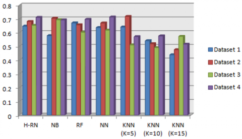
Figure 3. Recall results - phase 1
In Figure 3, we see clearly that the RF algorithm gives good results in data-set 1. On the other hand, H-RN gives the best recall rate for the third data set with a value of 0.711. This improvement is because our algorithm is based on the best parts of the two hybridized algorithms (RF and NB). Also, in the second and the last datasets, the recall rate of our algorithm is near to the best results compared to the other algorithms.
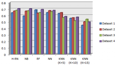
In Figure 4, the precision of H-RN is close to the best result of NB in datasets 2 and 3. In the last dataset, we notice that the precision of our algorithm (0.711) is almost similar to the best result (0.714) given by NN. The precision of our algorithm outperforms the precision of KNN (K=5, K=10, K=15) on all datasets except dataset 2 where the best result of KNN (k = 5) is 0.718, which is not very far from the best result (0.711) of our algorithm.
Figure 4. Precision results - phase 1
In this figure (Figure 5), we see clearly that H-RN dominates the KNN algorithm (K=5, K=10, K=15) in terms of F-measure for all datasets and the three other algorithms for datasets 2, 3, and 4 with a value of 0.668, 0.68, and 0.706 respectively. The raison for this enhancement is explained above in subsection 3.1. Also, H-RN is near to the best second results in the first dataset, however, RF gives the best F-measure.
Figure 5. F-measure results - phase 1
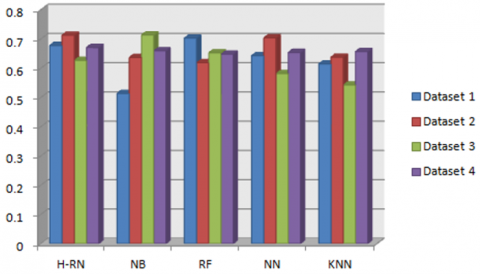
Figure 6. Accuracy results - phase 1
Table 3. Result of the average
|
Used algorithm |
Recall |
Precision |
F-measure |
|
H-RN |
0.667 |
0.673 |
0.673 |
|
Naïve-Bayes |
0.651 |
0.667 |
0.658 |
|
Random Forest |
0.674 |
0.657 |
0.664 |
|
Neural Network |
0.671 |
0.659 |
0.663 |
|
KNN (K=5) |
0.602 |
0.61 |
0.605 |
|
KNN (K=10) |
0.576 |
0.531 |
0.553 |
|
KNN (K=15) |
0.494 |
0.501 |
0.497 |
Figure 6 presents the accuracy results for all the algorithms. It is easy to notice in all datasets that H-RN outperforms KNN. Adding to that, in datasets 2 and 4, the accuracy dominance is for H-RN algorithm computation, but in the two other datasets, it has a second and third accuracy degree, respectively.
We notice from Table 3 that the H-RN algorithm gives the best results in the recall, precision and F-measure compared to KNN (K=5, K=10, K=15). In addition, it gives the best precision with a value of 0.673 and the best F-measure with a value of 0.673 compared to NB, RF, and NN. We also notice that both the NN, and RF algorithms give a good recall rate compared to NB, KNN, and H-RN.
4.2.2 The results for the second phase (with weather)
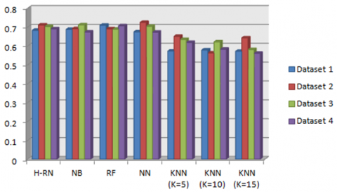
We see clearly in the Figure 7 that H-RN gives the best recall compared to KNN (K=5, K=10, K=15) in all datasets and the second good outcomes in datasets 1, 2, and 4 with a value of 0.742, 0.683, and 0.714, respectively, but in the third dataset, it is close to the tow first best results.
In this figure (Figure 8), H-RN provides the best precision in the four datasets in comparison with KNN (K=5, K=10, K=15) algorithm. It gives the second good precision in datasets 2 and 4 with a value of 0.711 and 0.691 respectively with regards to NB, RF, and NN, but in the first and the third dataset, it is near to the two first best precision values.
Figure 7. Recall results - phase 2
Figure 8. Precision results - phase 2
Figure 9. F-measure results - phase 2
Figure 9 represents the results of the F-measure which combines the results of the recall as well as the precision. We notice that H-RN gives the best results because it is confined between 0.691 and 0.718, on the other hand, the three other algorithms have less performance, i.e., NB gives results between 0.672 and 0.722, also NN gives results between 0.68 and 0.72.
Figure 10 represents the results of the accuracy for the four algorithms. We see that the H-RN dominates KNN and NN in most datasets, and the results are very close with a small dominance of the H-RN algorithm over NB and RF in the first and last datasets. The NN and RF algorithms provide the best accuracy for datasets 2 and 3, respectively.
Figure 10. Accuracy results - phase 2
Table 4. Result of the average
|
Used algorithm |
Recall |
Precision |
F-measure |
|
H-RN |
0.718 |
0.697 |
0.706 |
|
Naïve-Bayes |
0.705 |
0.691 |
0.697 |
|
Random Forest |
0.711 |
0.699 |
0.704 |
|
Neural Network |
0.711 |
0.694 |
0.702 |
|
KNN (K=5) |
0.7 |
0.619 |
0.657 |
|
KNN (K=10) |
0.62 |
0.586 |
0.603 |
|
KNN (K=15) |
0.563 |
0.589 |
0.576 |
From Table 4, we observe that the H-RN algorithm gives the best results in recall with 0.718 and F-measure with 0.706, as well as it is at second position in precision with 0.797 with a small difference of 0.02 compared to the first result of RF. In addition, we notice that the H-RN provides the best results in recall, precision, and F-measure vis-à-vis KNN (K=5, K=10, K=15). NN algorithm also gives good results compared to NB and RF.
From the detailed experimental results analysis of the recall, the precision, the F-measure, the accuracy, and the average by using the NB, the RF, the NN, the KNN, and the H-RN algorithms we conclude that there are two main results given by our hybrid algorithm:
(1) Phase 1 (without weather): produces an average rate accuracy of Recall, precision, and F-measure of 67.1%,
(2) Phase 2 (with weather): produces an average rate accuracy of Recall, precision, and F-measure of 70.7%, which is increased by 3.6% due to the enhancement in the rate of all evaluation criteria with the highest degree of recall (0.718), precision (0.697), and F-measure (0.706) compared to the results of phase 1 and also, we have an accuracy value improvement compared to the results of the other algorithms in both phases.
We can affirm that the best average scores are obtained by integrating the weather in the second phase of the recommendation process and also by the combination of both NB and RF algorithms. Technically, it can be concluded that weather conditions can improve the accuracy of the proposed method in recommender systems. In addition, H-RN is more precise than the other four algorithms (Naïve Bayes, Random Forest, Neural Network, and K-Nearest Neighbor).
4.3 Results and discussion with cross-validation
To assess the true accuracy of a model, calculating model accuracy is a critical part of any machine learning algorithm. The cross-validation technique allows us to compare different machine learning methods. This section discusses the results of the second experiment to measure and improve the accuracy of predictive algorithms and shows the usefulness of extracted context features (weather). This methodology is applied on four datasets (DS1, DS2, DS3, DS4) with five algorithms (H-RN, KNN (N=10, N=15), RF, NN, NB) without and with weather context (phase 1 (P1) and phase 2 (P2) respectively) where each model is trained on a subset of the initial data and predictions are formed for the other subset as detailed below.
The following tables summarize the cross-validated accuracy for five different machine learning methods, one time without randomness where the accuracy performed without weather and with weather like in Tables 5, 6, 7, and one time with the randomness inside of the cross-validation like in Tables 8, 9, 10.
The randomness in both cases is controlled via the random_state parameter, for instance, the random_state defaults to None in the case of without randomness.
4.3.1 K-fold cross-validation without randomness (WR)
Table 5. Accuracy of five machine learning methods on four data sets. Calculated with 5-fold cross-validation (WR)
|
Used algorithm |
H-RN |
KNN (K=10) |
KNN (K=15) |
RF |
NN |
NB |
|
|
DS1 |
P1 |
0.5972 |
0.5407 |
0.5216 |
0.6015 |
0.5733 |
0.5582 |
|
P2 |
0.6048 |
0.534 |
0.538 |
0.6042 |
0.5981 |
0.5840 |
|
|
DS2 |
P1 |
0.5672 |
0.5304 |
0.5281 |
0.5360 |
0.5619 |
0.5426 |
|
P2 |
0.5992 |
0.5607 |
0.5462 |
0.6017 |
0.6024 |
0.5933 |
|
|
DS3 |
P1 |
0.5982 |
0.6076 |
0.5933 |
0.5973 |
0.5810 |
0.5545 |
|
P2 |
0.6288 |
0.6198 |
0.6088 |
0.5288 |
0.6177 |
0.5952 |
|
|
DS4 |
P1 |
0.5841 |
0.5739 |
0.5804 |
0.5267 |
0.5759 |
0.5516 |
|
P2 |
0.5984 |
0.5967 |
0.5837 |
0.5995 |
0.5980 |
0.5963 |
|
Table 6. Accuracy of five machine learning methods on four data sets. Calculated with 10-fold cross-validation (WR)
|
Used algorithm |
H-RN |
KNN (K=10) |
KNN (K=15) |
RF |
NN |
NB |
|
|
DS1 |
P1 |
0.5913 |
0.5207 |
0.5087 |
0.6024 |
0.5683 |
0.5504 |
|
P2 |
0.5974 |
0.5193 |
0.5248 |
0.5947 |
0.5934 |
0.5895 |
|
|
DS2 |
P1 |
0.5584 |
0.5192 |
0.5116 |
0.5631 |
0.5475 |
0.5344 |
|
P2 |
0.5713 |
0.5273 |
0.5307 |
0.5646 |
0.6071 |
0.5767 |
|
|
DS3 |
P1 |
0.5870 |
0.5833 |
0.5544 |
0.5807 |
0.5749 |
0.5562 |
|
P2 |
0.6072 |
0.5973 |
0.5840 |
0.6166 |
0.5900 |
0.5862 |
|
|
DS4 |
P1 |
0.5992 |
0.5720 |
0.5648 |
0.5925 |
0.5408 |
0.5394 |
|
P2 |
0.5743 |
0.5834 |
0.5609 |
0.5933 |
0.5862 |
0.5907 |
|
Table 7. Accuracy of five machine learning methods on four data sets. Calculated with 15-fold cross-validation (WR)
|
Used algorithm |
H-RN |
KNN (K=10) |
KNN (K=15) |
RF |
NN |
NB |
|
|
DS1 |
P1 |
0.5737 |
0.5649 |
0.5420 |
0.5532 |
0.5771 |
0.5436 |
|
P2 |
0.5737 |
0.5662 |
0.5428 |
0.5628 |
0.5647 |
0.5429 |
|
|
DS2 |
P1 |
0.5582 |
0.5533 |
0.5287 |
0.5569 |
0.5560 |
0.5422 |
|
P2 |
0.5688 |
0.5615 |
0.5473 |
0.5705 |
0.5560 |
0.5585 |
|
|
DS3 |
P1 |
0.5609 |
0.5408 |
0.5545 |
0.5573 |
0.5578 |
0.5591 |
|
P2 |
0.5659 |
0.5482 |
0.5307 |
0.5631 |
0.5723 |
0.5571 |
|
|
DS4 |
P1 |
0.5541 |
0.5583 |
0.5462 |
0.5537 |
0.5619 |
0.5607 |
|
P2 |
0.5702 |
0.5533 |
0.5356 |
0.5770 |
0.5691 |
0.5433 |
|
4.3.2 K-fold cross validation with randomness (R)
You can clearly see that all machine learning methods have been able to improve the prediction accuracy from the weather phase in all cases, so the model has clearly learned something useful.
Table 8. Accuracy of five machine learning methods on four data sets. Calculated with 5-fold cross-validation (R)
|
Used algorithm |
H-RN |
KNN (K=10) |
KNN (K=15) |
RF |
NN |
NB |
|
|
DS1 |
P1 |
0.5934 |
0.5781 |
0.5537 |
0.5947 |
0.5814 |
0.5622 |
|
P2 |
0.6227 |
0.5844 |
0.5690 |
0.6132 |
0.6122 |
0.5937 |
|
|
DS2 |
P1 |
0.5807 |
0.5549 |
0.5380 |
0.5786 |
0.5965 |
0.5851 |
|
P2 |
0.5995 |
0.5607 |
0.5534 |
0.5955 |
0.6081 |
0.6054 |
|
|
DS3 |
P1 |
0.6172 |
0.6033 |
0.5764 |
0.6159 |
0.5840 |
0.5776 |
|
P2 |
0.6344 |
0.6091 |
0.5871 |
0.6350 |
0.6157 |
0.6108 |
|
|
DS4 |
P1 |
0.5906 |
0.5877 |
0.5641 |
0.5904 |
0.5937 |
0.5729 |
|
P2 |
0.5994 |
0.5963 |
0.5806 |
0.5969 |
0.6069 |
0.6033 |
|
Table 9. Accuracy of five machine learning methods on four data sets. Calculated with 10-fold cross-validation (R)
|
Used algorithm |
H-RN |
KNN (K=10) |
KNN (K=15) |
RF |
NN |
NB |
|
|
DS1 |
P1 |
0.5772 |
0.5600 |
0.5466 |
0.5922 |
0.5561 |
0.5418 |
|
P2 |
0.6182 |
0.5592 |
0.5476 |
0.6081 |
0.6133 |
0.5968 |
|
|
DS2 |
P1 |
0.5540 |
0.5327 |
0.5473 |
0.5545 |
0.5639 |
0.5472 |
|
P2 |
0.5937 |
0.5733 |
0.5362 |
0.5932 |
0.6072 |
0.6041 |
|
|
DS3 |
P1 |
0.5937 |
0.5961 |
0.5606 |
0.5989 |
0.5800 |
0.5869 |
|
P2 |
0.6049 |
0.5616 |
0.5831 |
0.6071 |
0.6208 |
0.6027 |
|
|
DS4 |
P1 |
0.5855 |
0.5633 |
0.5519 |
0.5908 |
0.5784 |
0.5757 |
|
P2 |
0.6002 |
0.5772 |
0.5644 |
0.5945 |
0.6043 |
0.5965 |
|
Table 10. Accuracy of five machine learning methods on four data sets. Calculated with 15-fold cross-validation (R)
|
Used algorithm |
H-RN |
KNN (K=10) |
KNN (K=15) |
RF |
NN |
NB |
|
|
DS1 |
P1 |
0.5534 |
0.5567 |
0.5372 |
0.5922 |
0.5693 |
0.5437 |
|
P2 |
0.6237 |
0.5961 |
0.5729 |
0.6209 |
0.6218 |
0.6196 |
|
|
DS2 |
P1 |
0.5481 |
0.5580 |
0.5439 |
0.5449 |
0.5551 |
0.5288 |
|
P2 |
0.6022 |
0.5837 |
0.5610 |
0.5986 |
0.6147 |
0.6111 |
|
|
DS3 |
P1 |
0.5790 |
0.5492 |
0.5522 |
0.5733 |
0.5608 |
0.5461 |
|
P2 |
0.6184 |
0.6033 |
0.5975 |
0.5945 |
0.6004 |
0.6059 |
|
|
DS4 |
P1 |
0.5962 |
0.5673 |
0.5497 |
0.5940 |
0.5830 |
0.5537 |
|
P2 |
0.6265 |
0.6052 |
0.5876 |
0.6222 |
0.6182 |
0.6094 |
|
Therefore, we evaluate each algorithm on test data with the settings: 5-cross validation, 10-cross validation and 15-cross validation without and random parameter.
Comparing the best accuracy for RF, NB, NN, KNN, and H-RN, we conclude that our proposed algorithm performs better in this study. H-RN provides recommendations with high quality for a huge amount of data. For instance, it achieves the best accuracy of 62.88 % for k-fold = 5 (without randomness parameter/with weather) over dataset 3 and 63,44% for k-fold = 5 (with a randomness parameter/with weather) over the same dataset. The bad values are in the range of k-fold=15 (54.81 %) delivered by the cross-validation of H-RN but the differences can still be somewhat large with KNN- K=15 (51.16%) on k-fold=10.
Comparing the accuracy results above with the accuracy results we calculated before in the split validation phase (subsection 4.2), we can see that the differences are sometimes quite high.
Ultimately the accuracy of the models in both split and cross-validation seem to vary significantly and this may be due to the time lag between train and test which causes some of the models to lose their ability to generalize as efficiently in future data (overfitting). From the results discussed above, k-fold cross-validation is the best possible method whenever one wants to validate the accuracy of a predictive model.
4.4 Statistical tests
In this subsection, we present an empirical study that involved: 1098, 2500, 200000, and 3112 users over 4 different datasets respectively (see section 1) and considered 6 at-tributes (see subsection 3.1), which implement 5 different state-of-the-art recommender algorithms. We measured the prediction quality of our system and compared our results against the statistical quality of the considered algorithms using accuracy metrics.
Using well-known techniques developed in the fields of information retrieval and machine learning, the quality of an RS is defined in terms of statistical metrics, error met-rics, and accuracy metrics. We perform the most popular tests in the field of the comparison of prediction algorithms. The ANOVA [42] is a hypothesis-testing technique used to determine whether three or more populations (or treatment) means are statistically different from each other. The diversity represents the truth between the elements of the recommendation [43].
We illustrate in the following the use of the One-way ANOVA and the diversity.
4.4.1 One way ANOVA
After the calculation of the ANOVA test, we will be able to compare the two variances and draw conclusions about:
- Hypothesis (H0): There is no significant difference in the AVG rating of items for the four sets of user groups.
- Hypothesis (H1): There is a significant difference in the AVG rating of items for the four sets of user groups.
We perform a one-way ANOVA using a value of α=0.05 (level of significance). To get the F-computed value, the following computations should be done: Sum of Square, Mean Square, Value of Ration.
Table 11. One Way ANOVA table
|
SOURCE |
Degrees of Freedom DF |
Sum of Squares SS |
Mean Square MS |
Value of Ratio Fc |
|
Treatment |
14 |
245 |
17.5 |
12.455 |
|
ERROR |
37 |
52 |
1.405 |
1.249 |
|
TOTAL |
51 |
297 |
18.905 |
13.704 |
According to Table 11, the F-computed (Fc) result is 12.455. We have to calculate the F-tabular (Ft) according to the following formula:
$F t=F(0.05, d f T, d f E)$ (10)
where df T represent the degree of freedom Treatment and df E represent the degree of freedom Error. Using the F Distribution table (The F distribution is a right-skewed distribution used most commonly in Analysis of Variance.), we cross the column value df T of 14 and the row value df E of 37 to get the critical value of Ft as follow: Ft = F (0.05, 14, 37) = 2.0921.
We see clearly that the Fc value is greater than the Ft value: Fc > Ft (12.455 > 2.0921), i.e., the difference in the calculated variations is sufficiently large, therefore, we can conclude that there is a difference in the population means. That is, we have sufficient evidence to reject H0 (disconfirm H0) which means that there is a significant difference in the rating of items for the four sets of user groups.
4.4.2 Diversity
The performance of the recommendation system is measured by the diversity of recommended items with each algorithm.
Table 12 demonstrates the diversity of the aforementioned algorithms in both case without and with weather context. It is clear that H-RN performed the best in terms of diversity in both without and with weather. The diversity of KNN (K=15) is also commendable. We conclude that the results of our algorithm are very rewarding.
Table 12. Diversity
|
Used algorithm |
without weather |
with weather |
|
H-RN |
1.208 |
1.472 |
|
KNN (K=5) |
0.182 |
1.130 |
|
KNN (K=10) |
1.067 |
1.354 |
|
KNN (K=15) |
1.206 |
1.466 |
|
Random Forest |
1.205 |
1.436 |
|
Neural Network |
0.216 |
1.149 |
|
Naïve-Bayes |
1.143 |
1.380 |
4.5 Error metrics
4.5.1 Root mean squared error (RMSE)
Table 13. RMSE
|
Used algorithm |
Dataset 1 |
Dataset 2 |
Dataset 3 |
Dataset 4 |
|
H-RN |
1.40 |
1.58 |
1.40 |
1.51 |
|
KNN (K=10) |
1.39 |
1.61 |
1.47 |
1.53 |
|
KNN (K=15) |
1.41 |
1.56 |
1.49 |
1.55 |
|
Random Forest |
1.44 |
1.52 |
1.48 |
1.54 |
|
Neural Network |
1.38 |
1.59 |
1.42 |
1.57 |
|
Naïve-Bayes |
1.41 |
1.47 |
1.49 |
1.59 |
4.5.2 Mean absolute error (MAE)
Table 14. MAE
|
Used algorithm |
Dataset 1 |
Dataset 2 |
Dataset 3 |
Dataset 4 |
|
H-RN |
0.000097 |
0.000108 |
0.000101 |
0.000094 |
|
KNN (K=5) |
0.000098 |
0.000096 |
0.000092 |
0.000103 |
|
KNN (K=10) |
0.000099 |
0.000108 |
0.000103 |
0.000097 |
|
KNN (K=15) |
0.000103 |
0.000098 |
0.000095 |
0.000101 |
|
Neural Network |
0.000125 |
0.000117 |
0.00012 |
0.000119 |
|
Naïve-Bayes |
0.000098 |
0.000098 |
0.000109 |
0.000097 |
Each cell above (Tables 13 and 14) shows the error test of each studied algorithm. Both MAE and RMSE express average model prediction error in units of the variable of interest. Both metrics are negatively-oriented scores, which means lower values are better. On average, the actual RMSE error is 1.58% higher for H-RN and 1.61% higher for KNN with k=10. However, the smaller value of the RMSE is returned by HRN in datasets 3 and 4 with 1.40 and 1.51 respectively by comparing KNN, NN, and NB.
H-RN classifier regains the lead in MAE in datasets 1 and 4. The High MAE occurs on NN with 0.000125. H-RN is placed in 3rd position in datasets 2 and 3 after KNN et NB.
In summary, from the above analysis, we can see that our proposition can definitely improve the prediction and the recommendation performance and decrease the value of RMSE and MAE.
4.6 Complexity study
The goal of complexity [44] is to measure the quality and the speed of an algorithm and allow a direct comparison between several algorithms according to the execution time or the number of instructions of each algorithm.
In the following, we will calculate the complexity of each algorithm used in our study. Table 15 represents the complexity of H-RN, KNN, RF, and NB.
The complexity of H-RN gives good results for N > 10000, while the complexity of KNN is low for N < 10000, knowing that the size of the datasets 1,2, and 4 of our study is greater than 10000. The complexity of RF is lower than our algorithm, but with a slight difference, as for NB, it has the same complexity with H-RN. Therefore, we can conclude that our algorithm can be used in practice because it is of polynomial complexity, efficient and very fast.
Table 15. Complexity of algorithms
|
Algorithm |
H-RN |
KNN |
RF |
NB |
|
Complexity |
O(n3+log(n)) |
O(log(n2)) |
O(n2 +2n) |
O(n3+log(2n)) |
The proposed approach is created to recommend the k-items that meet the user's needs. In other words, the challenge was focusing on predicting the recommendations that would be more suitable in visiting an appropriate tourist service. Machine learning algorithms can be useful in making predictions for the data.
The use of machine learning techniques allows to achieve and improve context-aware tourism recommendation system by analyzing not only the preferences, profile, and context of the user but also the context of the desired destination. Both model-based CF and memory-based CF are integrated into the proposed recommender model which is based on a broad array of ML algorithms. The combination of the two approaches yielded the best results in our work. Their merging was important because the first model was applied to a prediction and the other model was applied to a recommendation phase. Cross-validation is the best way to make full use of data without leaking information into the training phase. However, its only drawback is that the model validation takes more time than a single hold-out set.
The focus of this research is to improve the accuracy of predictions. Thus, an analysis of different ML algorithms such as Naïve Bayes, Random Forest, Neural Network, and KNN has been performed, as well as a detailed study of the proposed algorithm H-RN has been carried. For the experiment of this study, we have measured the recommendation accuracy through a series of experiments with real datasets. H-RN provides recommendations with high quality and performs the best in terms of accuracy and diversity (in both without and with weather) than KNN, RF, NB and NN. The recall, the precision, the F-measure and the average rating of H-RN give the best results in both split and cross-validation for all experiments. We can conclude that our approach can definitely improve the prediction and the recommendation performance and decrease the value of RMSE and MAE and the suggested algorithm can be used in practice because it is of polynomial complexity, efficient and very fast.
In future work, therefore, we will focus on improving the accuracy of recommendations by varying the k_item or combining our algorithm with clustering algorithms (X-means and Fuzzy C-means) to find the best prediction model. Further, we plan to extend our experiments with other public datasets, to review more in-depth analysis and improve the scalability and efficiency of this method. For additional research, extraction of other characteristics such as accompanying people (children, wife, friends, etc.) will enhance the recommendation quality, moreover, the more we add additional criteria in the compilation of the algorithm, the better results we get. To further boost results, a deep learning technique can be considered which combines various machine learning algorithms, and finally, some other metrics could be used as well such as the non-parametric and Bayesian tests to obtain a complete perspective of the comparison of the algorithms’ results.
[1] Mohri, M., Rostamizadeh, A., Talwalkar, A. (2018). Foundations of Machine Learning. MIT Press.
[2] Kulkarni, S., Rodd, S.F. (2020). Context Aware Recommendation Systems: A review of the state of the art techniques. Computer Science Review, 37: 100255. http://dx.doi.org/10.1016/j.cosrev.2020.100255
[3] Huang, Y., Bian, L.A. (2009). Bayesian network and analytic hierarchy process based personalized recommendations for tourist attractions over the internet. Expert Systems with Applications, 36(1): 933-943. http://dx.doi.org/10.1016/j.eswa.2007.10.019
[4] Wang, H. (2021). Research on personalized recommendation method of popular tourist attractions routes based on machine learning. International Journal of Information and Communication Technology, 18(4): 449-463. https://dx.doi.org/10.1504/IJICT.2021.115594
[5] Hayi, M.Y., Chouiref, Z. (2020). An improved optimization algorithm to find multiple shortest paths over large graph. 2020 Second International Conference on Embedded & Distributed Systems (EDiS)), Oran, Algeria, pp. 178-182. https://doi.org/10.1109/EDiS49545.2020.9296433
[6] Sánchez, P., Bellogín, A. (2021). Point-of-interest recommender systems: A survey from an experimental perspective. arXiv preprint arXiv:2106.10069.
[7] Debnath, M., Tripathi, P.K., Elmasri, R. (2016). Preference-aware successive POI recommendation with spatial and temporal influence. In International Conference on Social Informatics, Bellevue, WA, USA, pp. 347-360. http://dx.doi.org/10.1007/978-3-319-47880-7_21
[8] Weinberger, K.Q., Blitzer, J., Saul, L. (2005). Distance metric learning for large margin nearest neighbor classification. NIPS'05: Proceedings of the 18th International Conference on Neural Information Processing Systems, Cambridge, MA, United States, pp. 1473-1480.
[9] Ojagh, S., Malek, M.R., Saeedi, S. (2020). A social–aware recommender system based on user’s personal smart devices. ISPRS Int. J. Geo-Inf., 9(9): 519. http://dx.doi.org/10.3390/ijgi9090519
[10] Urner, J., Bucher, D., Yang, J., Jonietz, D. (2018). Assessing the influence of spatio-temporal context for next place prediction using different machine learning approaches. ISPRS Int. J. Geo-Inf., 7(5): 166. http://dx.doi.org/10.3390/ijgi7050166
[11] Barranco, M.J., Noguera, J.M., Castr, J., Martínez, L.A. (2012). Context-aware mobile recommender system based on location and trajectory. Advances in Intelligent Systems and Computing, 171: 153-162. http://dx.doi.org/10.1007/978-3-642-30864-2_15
[12] Gupta, R., Pandey, I., Mishra, K., Seeja, K.R. (2022). Recommendation system for location-based services. In: Applied Information Processing Systems, Advances in Intelligent Systems and Computing, Springer, 1354: 553-561. http://dx.doi.org/10.1007/978-981-16-2008-9_52
[13] Shafqat, W., Byun, Y.C. (2020). A context-aware location recommendation system for tourists using hierarchical LSTM model. Sustainability, 12: 4107. http://dx.doi.org/10.3390/su12104107
[14] Namahoot, C.S., Brückner, M., Panawong, N. (2015). Context-aware tourism recommender system using temporal ontology and naïve bayes. In Recent Advances in Information and Communication Technology, pp. 183-194. http://dx.doi.org/10.1007/978-3-319-19024-2_19
[15] Zhang, Z., Pan, H., Xu, G., Wang, Y., Zhang, P. (2017). A context-awareness personalized tourist attraction recommendation algorithm. Cybernetics and Information Technologies, 16(6): 146-159. http://dx.doi.org/10.1515/cait-2016-0084
[16] Uçar, T., Karahoca, A., Karahoca, D. (2019). NTRS: A new travel recommendation system framework by hybrid data mining. International Journal of Mechanical Engineering and Technology, 10(1): 935-946.
[17] Setiowati, S., Adji, T.B., Ardiyanto, I. (2018). Context-based awareness in location recommendation system to enhance recommendation quality: A review. International Conference on Information and Communications Technology (ICOIACT)), Yogyakarta, Indonesia, pp. 90-95. http://dx.doi.org/10.1109/ICOIACT.2018.8350671
[18] Paradarami, T.K., Bastian, N.D., Wightman, J.L. (2017). A hybrid recommender system using artificial neural networks, Expert Syst. Appl., 83: 300-313. http://dx.doi.org/10.1016/j.eswa.2017.04.046
[19] Kumar, S., Singh, M. (2019). A novel clustering technique for efficient clustering of big data in Hadoop Ecosystem. Big Data Mining and Analytics, 2(4): 240-247. http://dx.doi.org/10.26599/BDMA.2018.9020037
[20] Pang, L., Liu, Y. (2020). Construction and application of a financial big data analysis model based on machine learning. Rev. d'Intelligence Artif., 34(3): 345-350. http://dx.doi.org/10.18280/ria.340313
[21] Fenanir, S., Semchedine, F., Baadache, A. (2019). A machine learning-based lightweight intrusion detection system for the internet of things. Rev. d'Intelligence Artif., 33(3): 203-211. http://dx.doi.org/10.18280/ria.330306
[22] Liping, C., Yujun, S., Saeed, S. (2018). Monitoring and predicting land use and land cover changes using remote sensing and GIS techniques-A case study of a hilly area, Jiangle, China, PLoS One, 13(7): 0200493. http://dx.doi.org/10.1371/journal.pone.0200493
[23] Voulodimos, A., Doulamis, N., Doulamis, A., Protopapadakis, E. (2018). Deep learning for computer vision: A brief review. Computational Intelligence and Neuroscience, 2018: 7068349. http://dx.doi.org/10.1155/2018/7068349
[24] Jiao, C. (2020). Big data mining optimization algorithm based on machine learning model. Rev. d'Intelligence Artif., 34(1): 51-57. http://dx.doi.org/10.18280/ria.340107
[25] Mueller, J.P., Massaron, L. (2016). Machine Learning for Dummies, John Wiley & Sons.
[26] Zhang, S., Yao, L., Sun, A., Tay, Y. (2019). Deep learning based recommender system: A survey and new perspectives. ACM Computing Surveys (CSUR), 52(1): 3285029. http://dx.doi.org/10.1145/3285029
[27] Nilashi, M., Bagherifard, K., Rahmani, M., Rafe, V. (2017). A recommender system for tourism industry using cluster ensemble and prediction machine learning techniques, Computers & Industrial Engineering, 109: 357-368. http://dx.doi.org/10.1016/j.cie.2017.05.016
[28] Paradarami, T.K., Bastian, N.D., Wightman, J.L. (2017). A hybrid recommender system using artificial neural networks. Expert Syst. Appl, 83: 300-313. http://dx.doi.org/10.1016/j.eswa.2017.04.046
[29] Giglio, S., Bertacchini, F., Bilotta, E., Pantano, P. (2020). Machine learning and points of interest: Typical tourist Italian cities. Current Issues in Tourism, 23(13): 1646-1658. http://dx.doi.org/10.1080/13683500.2019.1637827
[30] Abbasi-Moud, Z., Vahdat-Nejad, H., Sadri, J. (2021). Tourism recommendation system based on semantic clustering and sentiment analysis. Expert Systems with Applications, 167: 114324. http://dx.doi.org/10.1016/j.eswa.2020.114324
[31] Renjith, S., Sreekumar, A., Jathavedan, M. (2020). An extensive study on the evolution of context-aware personalized travel recommender systems. Information Processing & Management, 57(1): 102078. http://dx.doi.org/10.1016/j.ipm.2019.102078
[32] Portugal, I., Alencar, P., Cowan, D. (2018). The use of machine learning algorithms in recommender systems: A systematic review. Expert Systems with Applications, 97: 205-227. http://dx.doi.org/10.1016/j.eswa.2017.12.020
[33] Breiman, L. (2001). Random forests. Machine Learning, 45(1): 5-32.
[34] Panagiotakis, C., Papadakis, H., Fragopoulou, P. (2021). A dual hybrid recommender system based on SCoR and the random forest. Computer Science and Information Systems, 18(1): 115-128. https://doi.org/10.2298/CSIS200515046P
[35] Kbaier, M.E.B.H., Masri, H., Krichen, S.A. (2017). Personalized hybrid tourism recommender system. IEEE/ACS 14th International Conference on Computer Systems and Applications (AICCSA)), Hammamet, Tunisia, pp. 244-250. http://dx.doi.org/10.1109/AICCSA.2017.12
[36] Wan, L., Hong, Y., Huang, Z., Peng, X., Li, R. (2018). A hybrid ensemble learning method for tourist route recommendations based on geo-tagged social networks. International Journal of Geographical Information Science, 32(11): 2225-2246. https://doi.org/10.1080/13658816.2018.1458988
[37] Saravanan, R., Sujatha, P. (2018). A state of art techniques on machine learning algorithms: A perspective of supervised learning approaches in data classification. Second International Conference on Intelligent Computing and Control Systems (ICICCS)), Madurai, India, pp. 945-949. http://dx.doi.org/10.1109/ICCONS.2018.8663155
[38] Xu, Y., Goodacre, R. (2018). On splitting training and validation set: A comparative study of cross-validation, bootstrap and systematic sampling for estimating the generalization performance of supervised learning. Journal of Analysis and Testing, 2(3): 249-262. http://dx.doi.org/10.1007/s41664-018-0068-2
[39] Powers, D.M. (2020). Evaluation: from precision, recall and F-measure to ROC, informedness, markedness and correlation. arXiv preprint arXiv:2010.16061. https://doi.org/10.48550/arXiv.2010.16061
[40] Demšar, J. (2006). Statistical comparisons of classifiers over multiple data sets. The Journal of Machine Learning Research, 7: 1-30.
[41] Botchkarev, A. (2018). Performance metrics (error measures) in machine learning regression, forecasting and prognostics: Properties and typology. arXiv preprint arXiv:1809.03006.
[42] Kim, H.Y. (2014). Analysis of variance (ANOVA) comparing means of more than two groups. Restorative Dentistry & Endodontics, 39(1): 74-77. http://dx.doi.org/10.5395/rde.2014.39.1.74
[43] Matevz, K., Tomaz, P. (2017). Diversity in recommender systems - A survey. Knowledge-Based Systems, 123: 154-162. https://doi.org/10.1016/j.knosys.2017.02.009
[44] Hartmanis, J., Stearns, R.E. (1965). On the computational complexity of algorithms. Transactions of the American Mathematical Society, 117: 285-306. http://dx.doi.org/10.1090/S0002-9947-1965-0170805-7