Sameer Kaul | Sheikh Amir Fayaz | Majid Zaman* | Muheet Ahmed Butt
© 2022 IIETA. This article is published by IIETA and is licensed under the CC BY 4.0 license (http://creativecommons.org/licenses/by/4.0/).
OPEN ACCESS
Decision trees are one of the oldest and most used (successful) machine learning algorithms. Over the years various modifications of decision tree have been proposed and implemented. In the recent past decision trees has many upgraded versions, including Random forests (RF), Random trees (RT), Distributed Decision trees (DDT) and Model Trees (MT) which are readily used nowadays. In this paper effort has been made to determine whether decision trees in its core form are still relevant in the era or obsolete.
decision tree, random forest, distributed decision trees, model trees
Decision tree is a binary tree that recursively splits the dataset until we are left with the pure leaf nodes which defines the decision i.e. the data with only one type of class. In decision tree there are two kinds of nodes: decision nodes and leaf nodes. The former one contains a condition to split the data and the latter one helps us to decide the class of a new data point. Since, decision tree internally is a bunch of nested if-else statements and we still consider it as a Machine learning approach because there are many possible splitting conditions which need to learn which feature to take and the corresponding correct threshold values to optimally split the data. The goal of a decision tree model is to get the pure leaf nodes and for that the model iteratively splits the data until all the nodes are processed. This is the theoretical approach about the working of decision tree [1].
Mathematically, it can be processed using information theory. More precisely the model will choose the split that maximizes the information gain. To calculate the information gain we first need to understand the information contained in a state. Imagine we are predicting the class of randomly picked points. Only half of time we will be correct, i.e. the state has the highest uncertainty or impurity. The way to quantify this is to use the entropy, i.e. if the entropy value is highest then we are uncertain about the randomly picked points and then it needs more bits to describe its state. The entropy can be calculated as (1):
Entropy $=\sum-p_{i} \log p_{i}$ (1)
Here, $p_{i}$ is the probability of class $i$.
The highest possible value of entropy for a binary class is 1 and the lowest value for the entropy is 0 (pure node). To find the information gain corresponding to a split we need to subtract the combined entropy of child node from the entropy of parent nodes as shown below (2):
$I G=E_{(\text {parent })}-\sum w_{i} E_{(\text {child })_{i}}$ (2)
Here, $w_{i}$ is the relative size of the child node with respect to the parent node. In reality the node compares the every possible split and takes the one with the maximum information gain. So, the model traverses through every possible feature and feature value to search for the best feature and the corresponding threshold. Thus, we can point out with this that decision tree is a greedy algorithm where it selects the best split that maximizes information gain. It does not backtrack and change a previous split and this doesn’t guarantee that we will get most optimal set of splits but greedy search makes our training a lot faster and it works really good despite of its simplicity [2].
Many decision trees inducers follow the top-down approach which includes ID3, C4.5, CART, CHAID Quest etc. Some of them consist of two abstract phases: growing and pruning (C4.5 and CART) phases and some of the other inducers implement growing phase only. Some of the decision tree inducers are described below [3].
2.1 Iterative Dichotomiser 3 (ID3)
This is considered as one of the simplest algorithms where information gain is used as its one of the splitting criteria. The node with highest information gain will be chosen as the splitting node. In this approach pruning and numeric data can be handled easily but this algorithm may not be used to handle the missing values [4].
2.2 Classification and Regression Tree (CART)
The main characteristic of this decision tree inducer is that it is used to construct the decision tree based on the towing criteria. This type of inducer enables to use the prior probability distribution and can consider misclassification cost in its original form of tree induction. CART algorithm is used to predict the real number at the leaf nodes in place of class because this algorithm has the ability to generate regression trees [4].
2.3 QUEST
This type of algorithm is quick and unbiased efficient algorithm. This algorithm supports univariate and linear combinations of the split where the association of input and output target variable is calculated using ANOVA F-testing or Pearson’s testing for ordinal and nominal data respectively. For optimal splitting a basic approach of Quadratic Discriminant Analysis (QDA) is used on the input attributes. This type of tree-based approach uses cross validations for pruning purposes to remove the complexity of the original tree, without affecting the overall performance [4].
2.4 CHAID
In earlier 1980’s, this algorithm was only designed to handle the nominal values. Significant difference value is calculated using statistical testing which depends on the value present at the target attribute. It follows the QUEST testing approach i.e. for nominal data: Pearson testing is used, for ordinal data: Likelihood testing is performed and for continuous data: F-testing is used. CHAID lacks pruning feature but it can handle missing data efficiently.
There are numerous other decision trees inducers available like: C4.5, AID, MAID, THAID, CAL5, LMTD, PUBLIC, MARS, and FACT etc. These inducers differ slight in their working. Some of them differ in pruning, and some differ in testing criteria and some other works on multivariate data and so on [4].
Since all the decision tree inducers more or less follow the same procedure to construct the decision tree from a given set of data. The major goal is to optimize the output results which can be done by improving the accuracy measure and by reducing the error content. Furthermore, it is not only to increase the accuracy measure but it also depends on the time and space complexity of the algorithm and the number of rules generated in optimizing the overall results. This may include the pruning factors of the algorithm as well. Thus, finding out the best optimized algorithm is a quite hard task as we don’t have to check the accuracy measure only but other factors are also taken into consideration [5]. The other factors include recall, sensitivity, specificity, Cohen kappa, F-measure etc. These factors are basically used for information retrieval and are used to evaluate the performance in determining the strength of an algorithm. In the field of data sciences these statistical factors specifically allow us to visualize the performance of an algorithm. Some of these machine learning measures are calculated in this study and are shown in below table (Table 2).
It has been proposed that finding the minimal decision tree from the training set is NP-hard and constructing the minimal decision tree from the expected set of outcomes is NP-complete. Furthermore, it has been proposed that finding the optimal decision tree is also a NP-hard problem.
Optimal decision tree construction is only feasible for small task where smaller set of data is present or where smaller problems are taken into account. Thus, constructing a decision tree using above mentioned decision tree inducers may not be sufficient for optimizing the performance alone.
3.1 Potentials with decision tree inducers
3.2 Problems with decision tree inducers
In this study we have used the geographical dataset of Kashmir province which has been collected from Indian Metrological Department Pune [10]. The dataset contains 5 attributes namely: Maximum temperature (℃), minimum temperature (℃), Humidity@12 (Humidity measured at 12 A.M), humidity@3 (Humidity measured at 3 P.M), and the target attribute rainfall. The snapshot of the data is shown below (Table 1).
Table 1. Geographical dataset
|
Max_Temp |
Min_Temp |
Humidity@12 |
Humidity@3 |
Rainfall |
|
7.5 |
1 |
81 |
99 |
Y |
|
16.8 |
12.5 |
98 |
79 |
Y |
|
16.5 |
11.2 |
96 |
66 |
Y |
|
19.5 |
14 |
96 |
98 |
N |
|
25.7 |
12.9 |
96 |
72 |
Y |
|
30.7 |
15.8 |
86 |
98 |
N |
|
15.5 |
12.8 |
94 |
88 |
Y |
|
20.5 |
16.4 |
73 |
98 |
Y |
|
19.6 |
13 |
91 |
73 |
Y |
|
20 |
14.5 |
61 |
98 |
Y |
|
13 |
4.6 |
68 |
64 |
N |
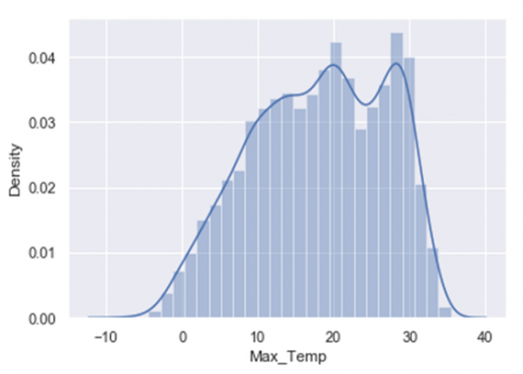
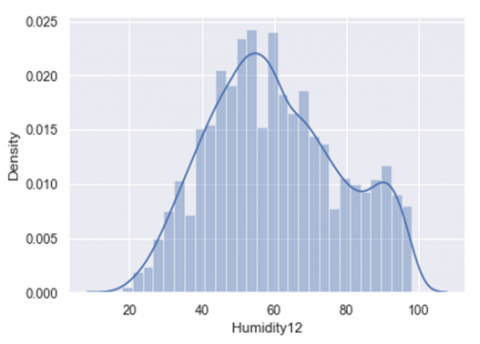
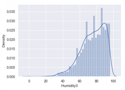
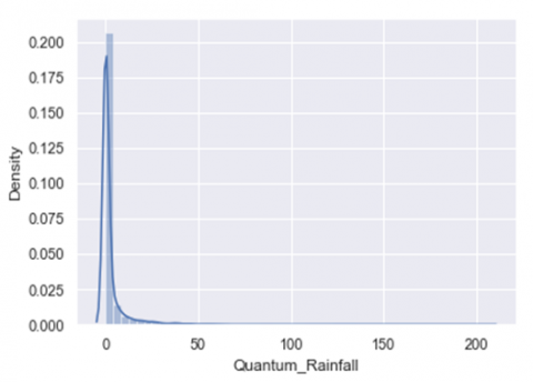
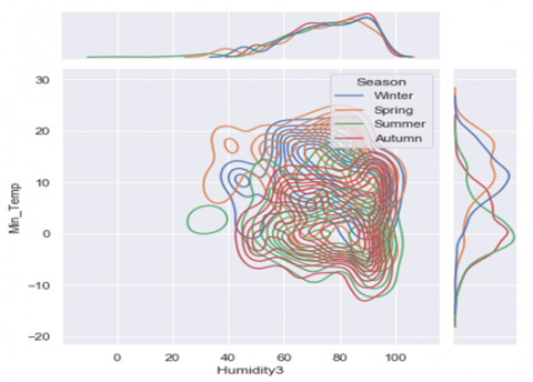
Data visualization is the process of taking raw data in a powerful way and transforming it into beautiful & ascetic graphs, charts, images & even videos that explain the numbers and allow us to gain insights from it. Finding insights from the data is extremely hard, so this is the way where data visualization can be widely used in order to contribute in developing an accurate, robust pattern & spot trends from the data. The multivariate dataset which is to be visually analyzed is of high dimensionality and these parameters are correlated in some way. The underneath figures (Figure 1, Figure 2, Figure 3, Figure 4) shows the relationship among different parameters including Humidity, Temperature, Season and rainfall based on various plots using various python libraries like Matplotlib, Seaborn, Ggplot in which each having different advantages. These python libraries are used in this study to visualize the geographical data of Kashmir province, its correlation among attributes and densities etc. [10].
(a) Data distribution of Min_Temp against the density distribution
(b) Data distribution of Max_Temp against the density distribution
(c) Data distribution of Humidity12 against the density distribution
(d) Data distribution of Humidity3 against the density distribution
(e) Data distribution of Target Variable (Quantum_Rainfall) against the density distribution
Figure 1. Univariate distribution of data
In Figure 1 (a-e) data distribution of different attributes against the particular density distribution has been shown. In the normal histogram we have a grouped data of fixed number of categories and from that we are able to see the density of where the most of the data is occurring. If we were to use more and more number of categories, instead of limited categories, we would be able to create a perfect curve by tops of each bar with a smooth line. This smooth curve is called a density curve and with this we will be able to know how much amount of total area that falls under the curve within that interval.
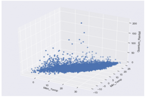
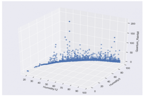
(a) 3D- Scatter plotting of the attribute Max-Temp, Min_Temp and the target attribute Rainfall
(b) 3D- Scatter plotting of the attribute Max-Temp, Min_Temp and the target attribute Rainfall
Figure 2. 3D Scatter plot of various attributes of the dataset
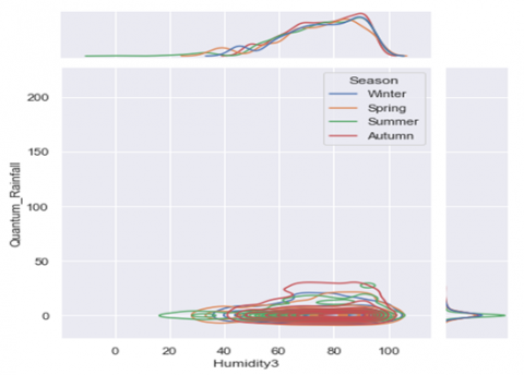
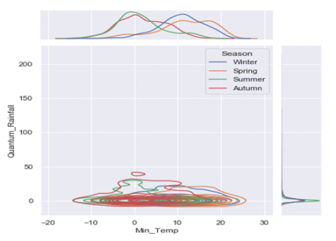
Here, in Figure 3(a&b) effect of rainfall on attributes are irrespective of quantum of rainfall and vice-versa.
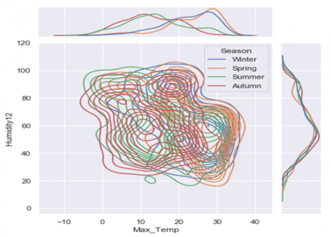
(a) Bivariate and Univariate graph of attribute Humidity12 & Max_Temp
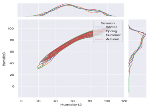
(b) Bivariate and Univariate graph of attribute Humidity3 & Humidity12
(c) Bivariate and Univariate graph of attribute Max_Temp&Humidity3
(d) Bivariate and Univariate graph of attribute Quantum_Rainfall&Humidity3
(e) Bivariate and Univariate graph of attribute Quantum_Rainfall & Min_Temp
Figure 3. 3D Binary and Univariate distribution of various attributes of the dataset
In Figure 3 (a-e) the horizontal and vertical co-ordinates remain the same, e.g. in Figure 3(a) the horizontal co-ordinate, in front view depicts the max_temp and the vertical co-ordinate shows the Humidity measure at 3 P.M. This process is same for all other attributes.
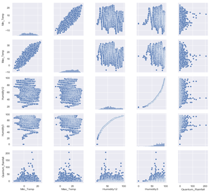
Figure 4. Distribution of single variables and relationships between other variables of the Dataset
The major advantage of using plots in data visualization is that they contain various visual dimensions that human can distinguish effectively and pre-attentively. Besides, the outcomes are generally more engaging and aesthetic that are more attractive and favorable, independent of what type of textures are being used.
5.1 Random Forest (RF)
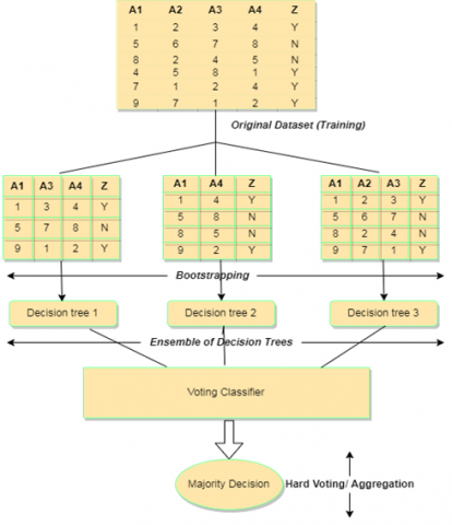
Random forest is considered as the most popular supervised machine learning algorithm which is capable of implementing both classification and regression tasks. It is an ensemble method that is used to train the different decision trees in a parallel manner with bootstrapping which is followed by the aggregation. This process is called as Bagging in which number of different decision trees are trained in different subsets and for the final decision it aggregates the individual decisions from the different individual decision trees and consequently it shows good generalization. Implementation of RF classifier on a dataset that has four features (A1, A2, A3, and A4) and two classes (Z = Y and N). RF classifier is an ensemble method that trains several decision trees in parallel with bootstrapping followed by aggregation as shown in Figure 5. Each tree is trained on different subsets of training sample and features [11].
Figure 5. Random Forest Model
The major advantage of using random forests over decision tree approach is that it can handle the missing values and maintains the accuracy for missing data. It also handles the large set of data with higher dimensionalities without over-fitting the model. i.e. it inclines to outrange most of the other classification methods with respect to the accuracy without over-fitting [11].
Thus, if the number of trees increases the overfitting problem will reduce and thus converges the generalization error. In other words, reducing the number of analytical variables can results in weakening of each individual tree of the model, which leads to reduce the correlation between the trees and improve the accuracy of the model. Therefore, it is necessary to choose a large number of trees and to minimize the generalization error by optimizing the number of predictive variables [11].
In building the random forest, time and space complexity play a major role in its performance. Initially, before building a random forest, we have to define the number of sub-trees a random forest contains, and this can be denoted as "$n$-tree", where $n$ defines the total number of sub-trees. We further need to take care of the number of variables we want to sample at each node, and it can be denoted by "$m$-try", where "$m$" denotes the number of variables or attributes.
Thus, in order to build one tree with "m-try" variable, the complexity would be:
$\mathrm{O}(\operatorname{mtry} * \mathrm{n} \log (\mathrm{n}))$
Furthermore, if the number of sub-trees be "n-tree", then the complexity would be:
$\mathrm{O}($ ntree $*$ mtry $* \operatorname{nlog}(\mathrm{n}))$
where $\mathrm{n} \log (\mathrm{n})$ is assumed as the depth of the tree and is treated as the worst case complexity scenario.
5.2 Distributed Decision Trees (DDT)
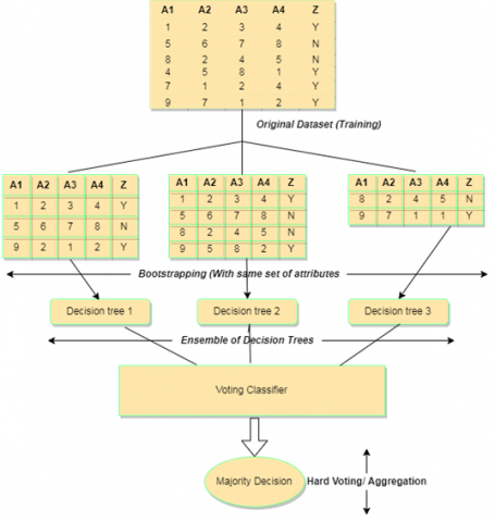
In practice, amongst the diverse situations for classification involving the large sets of data including big datasets where the volume of data is huge to manage and evaluate. In such situations a distributed implementations are carried out, i.e. the concept of distributed decision trees are implemented where a particular number of decision trees are generated based on the number of partitions carried out in the input data [12]. Suppose if there are n number of partitions in the input data then it will result in the n number of sub trees and the overall prediction and the classification are carried out on the basis of voting i.e. the individual performances or predictions of the sub trees are recorded and the final prediction and classification is calculated based on these individual performances by implementing the concept of voting technique [12], .i.e. Number of Decision Trees (Models) = n, Where n is the number of splits/partitions.
Figure 6. Distributed Decision Tree Model
The graphical representation of the Distributed Decision Tree model is shown in Figure 6.
In distributed decision trees the prediction of one sub tree is independent on other sub trees, i.e. all the sub trees predict individually and then voting technique is applied in which the majority of the decisions will be chosen as the final output for the prediction. Suppose if there are 1000 entries present in the original dataset and the data is split into 5 partitions i.e. 5 decision trees will be created and if the target attribute is binary classified [0,1] and every decision tree either predicts 0 or 1. Then the final output will be the majority count of 0 or 1 from all the sub trees [13].
5.2.1 Steps for implementing distributed decision tree
The distributed decision tree follows a simple approach in its implementation process. In order to implement the distributed decision tree on a particular set of data, it needs to be divided into a certain number of partitions based on a particular attribute. Suppose the data used in this paper originally contained the station_ID as one of its attributes. The station_ID contains discrete values of three stations (42044, 42027, and 42026) [11], and these three stations belong to the three different regions (south zone, north zone, and central zone) of the UT of the Jammu and Kashmir region of India. Thus, we have three subsets of original data, and in order to check the individual performances of these subsets, we need the concept of distributed decision trees. A voting classifier was used to validate the prediction's final output value. A voting classifier declares the majority value of "Yes" or "No" as the final output of the prediction class. Suppose two of the subsets arrive with a decision of yes, and one subset arrives with a decision of no. Then, the final output value for the prediction class will be the majority one, i.e., yes.
5.3 Model Trees (MT)
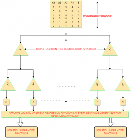
Model tree is another decision tree extension algorithm where a step wise implementation is carried out to construct a tree. This step wise implementation follows a two level approach where at first level any simple decision tree inducer (C4.5) is used for the construction of decision tree and latter at second level model tree functions are used at the leaf nodes [13].
For example, The C4.5 builds a decision tree based on top-down, recursive and “divide and conquer” approach. It constructs the decision tree based on the information gain theory concept in which the splitting attribute which has the highest information gain ratio will be chosen as the splitting node parameter. The information gain can be defined as the reduction in the entropy after the dataset is divided on an attribute. In the next step the regression at each leaf node is applied which can result in the pruning of the original decision tree inducer (C4.5). Pruning of trees at interior nodes are then replaced by the regression plane instead of a constant value which can also results in the rules generated by the LMT. This is usually done when the branches of the tree are not useful in the later stages. The main advantage of this step is that it reduces the level of complexity of the classifier without affecting the overall performance of the original tree. There are two primary strategies for pruning:
1) With reduced error pruning in which the most popular class replace the nodes and starting at leaves. This approach is used to simplify the data and increasing speed. M5 model tree follows a greedy approach for minimization of errors at each internal node in which Standard deviation reduction is calculated one node at a time and is given by (3):
$S D R=\frac{S D(T)-\sum S D\left(T_{i}\right)\left|T_{i}\right|}{|T|}$ (3)
Pruning of trees at interior nodes are then replaced by the regression plane instead of a constant value which can also results in the rules generated by the M5 Model tree. This is usually done when the branches of the tree are not useful in the later stages. The main advantage of this step is that it reduces the level of complexity of the classifier without affecting the overall performance of the original tree.
2) With cost computing pruning (CCP) where it is used to define the cost-complexity measure of the tree [13, 14]. Logistic model tree (LMT) follows cost-complexity pruning approach in order to reduce the variance of the model and with this, it will have better performance on different types of data. This can be computed as (4):
CCP $=\frac{\operatorname{err}(\operatorname{prune}(T, t), S)-\operatorname{err}(T, S)}{\mid \text { leaves }(T)|-| \text { leaves }(\operatorname{prune}(T, t)) \mid}$ (4)
where, $\operatorname{err}(T, S)$ is the error rate of tree T over dataset $S$, and ( $\operatorname{prune}(T, t), S)$ is the tree obtained by pruning the sub trees $t$ after the regression is applied on the tree $T$.
The basic methodology of Model trees is shown in below Figure 7.
Figure 7. Model Tree
Model trees can predict a numeric value like an ordinary regression tree works, that is defined over a permanent number of numeric or nominal parameters but distinctly model trees construct a piecewise or Hamiltonian linear estimations to the target function [15]. Thus, the resultant model tree constructs a tree with the logistic or linear regression functions at the leaf nodes. The principal advantage of using this machine learning methodology is that it acts as a white box learning model where each and every step is defined by the mathematical expression that shows the dependencies between the attributes. Furthermore, model trees can perform feature selection implicitly, data preparation becomes an easy process i.e. less effort needs to be taken while performing data preparation [16-27], and it can handle missing values also.
The basic methodology of decision tree inducers (ID3, CART, QUEST, C4.5) and decision tree extensors (RF, DDT, MT) remains the same. However, the latter versions are customized for generating better results.
6.1 Implementing decision tree inducers
Building decision tree is a straight forward approach where it can be constructed by using ID3, CART, QUEST, and C4.5 and so on. All of them more or less follow the same approach but the difference lies in the splitting of the nodes.
Entropy: $H(S)=-p_{(+)} \log _{2} p_{(+)}-p_{(-)} \log _{2} p_{(-)}$ (5)
where, $S=$ subset of training examples and $p_{(+)}, p_{(-)}$are the percentages of positive and negative samples.
The information gain can be defined as the reduction in the entropy after the dataset is divided on an attribute. To calculate the information gain of an attribute a comparison of the entropy of the dataset after and before a transformation needs to be done [17]. The attribute with the highest information gain will lead to the construction of a decision tree by acting as a splitting node with the homogenous branches (6).
$\operatorname{Gain}(S, A)=H(S)-\sum_{A} \frac{\left|S_{v}\right|}{|S|} H S_{v}$ (6)
where,
$V$ is the possible value of $A$;
$S=$ Set of examples;
$S_{v}$ denotes subset where $X_{A}=V$.
The above information Gain formula is an iterative process where it calculates the information gain of each node at every level of the decision tree until all the nodes are processed.
$\operatorname{GINI}(D)=1-\sum_{i=1}^{m} p i^{2}$ (7)
where, D is the binary split on A into D1, D2 as shown below (8):
$G I N I_{A}(D)=\frac{\left|D_{1}\right|}{|D|} G I N I\left(D_{1}\right)+\frac{\mid D_{2 \mid}}{|D|} \operatorname{GINI}\left(D_{2}\right)$ (8)
This process continues recursively and the attribute with the less impurity (Minimum GINI coefficient) is chosen as splitting attribute. Thus, from Eqns. (5) and (6), we get (9):
$G I N I_{A}=G I N I(D)-G I N I_{A}(D)$ (9)
Furthermore, same approach is used in other decision tree inducers for the construction of decision trees. The various criteria’s for splitting the nodes in other decision tree inducers include: DKM Criteria, Normalized Impurity based criteria, Distance measure criteria, Binary Criteria, Towing criteria, Orthogonal Criterion (ORT), Kolmogorov-Smirnov Criterion, AUC-Splitting Criteria etc. [18].
6.2 Implementing decision tree extensors
This approach follows the same strategy in the construction of decision trees but these are upgraded to another level where it can be proven more efficient as simple decision tree inducers based on the data used for the operation.
The implementation strategy of decision trees extensors is well described in the section 5.
In this approach the experimental evaluation of some decision tree inducers and decision tree extensors has been carried out on the geographical data of Kashmir province. For the simulation study an open source data Analytics tool called KNIME, has been used. The experiment was carried out on the 70-30 ratio in which 70% was used as the training set and 30% was used for testing purposes. The dataset consists of 4 independent continuous parameters which includes minimum and maximum temperatures, Humidity at two different intervals and one dependent variable rainfall with continuous values [19].
Table 2. Accuracy statistics
|
Algorithm |
ID3 |
SVM |
KNN |
Fuzzy DT |
DDT |
C4.5 |
LMT |
|
Model |
30-70 |
30-70 |
30-70 |
30-70 |
30-70 |
30-70 |
30-70 |
|
Accuracy |
80.12 |
81.07 |
78.94 |
77.75 |
78.46 |
66.99 |
87.23 |
|
No. of Rules |
51 |
--- |
--- |
--- |
21 |
55 |
10 |
|
Error |
19.87 |
18.92 |
21.05 |
22.24 |
21.54 |
33.01 |
12.77 |
|
Precision |
0.812 |
0.845 |
0.848 |
0.841 |
--- |
0.880 |
0.892 |
|
Recall |
0.938 |
0.897 |
0.857 |
0.846 |
--- |
0.726 |
0.973 |
|
Cohen Kappa |
0.456 |
0.519 |
0.485 |
0.458 |
--- |
-0.022 |
0.102 |
|
F-measure |
0.87 |
0.871 |
0.853 |
0.844 |
--- |
0.796 |
0.931 |
|
Specificity |
0.938 |
0.897 |
0.857 |
0.846 |
--- |
0.238 |
0.098 |
|
Sensitivity |
0.938 |
0.897 |
0.857 |
0.846 |
--- |
0.726 |
0.973 |
In order to check the performances of both DT inducers and DT extensors individual implementation has been carried out on same set of data. It was observed that all the algorithms show more or less same performance but Model trees shows better performance as compared to other algorithms [20].
Table 2 shows the individual performances of the various algorithms (Both Inducers and Extensors) used in predicting the rainfall of Kashmir province.
We can confirm from the above table that the number of rules in LMT are only 10 with an accuracy of 87.23%. But this doesn’t define that LMT always produces better results than any traditional decision tree inducers [21-25]. The performance measure of any algorithm depends on the type of data on which the work has been carried out [26]. In this study, although the accuracy has been increased in logistic model tree but internally the working of logistic model tree is totally dependent on methodology of basic decision tree inducer (ID3, C4.5 etc.). So, it is very tough to say that decision tree in its original form has lost its applicability or capability.
Decision tree in its core form is the most used machine learning algorithm. Over the past decades various modifications have been proposed on decision tree including: Random Forest, Distributed Decision trees and Model trees and these modifications have produced desirable results. So, the question arises “has the decision tree lost its relevance?” And is decision tree reduced to benchmark algorithm which will (primarily) be used for training and educating but in real world its modified version will be used instead.
In this paper effort has been put to answer the relevance of decision trees in current machine learning era. Accordingly, Decision tree and its modifications were implemented on geographical data of Kashmir province having 5 attributes and the results generated are shown in Table 2. The result put the argument to rest and proves the decision tree in its core form continues to be as relevant as its extensors like: Random forests, Distributed Decision trees and Model trees.
All the tree flavors, starting from the core decision tree to ensemble approaches (multiple decision trees, distributed decision trees, and model trees) have been implemented on one set of data. The purpose was to check the performance of individual decision trees and all other decision tree extensors. After checking the performance measures, the question arises whether the performance of the decision tree extensors improved over the original decision tree or not. Does the original decision tree performance hold up or has it now become a yardstick algorithm? While implementing, we evaluated that the decision tree in its very core form is still upheld because, in many cases, the original decision tree performs better than its extensors like random forest, DDT, and MT. Thus, in this study, we conclude that datasets determine the applicability and audibility of an algorithm.
Performance of an algorithm be it Decision Tree, or its modifications/ up-gradations is primarily specific to dataset and no algorithm can be generalized. The applicability of an algorithm is primarily dependent on the type of the dataset used. Thus, in this study we conclude that dataset determine the applicability and audibility of an algorithm in generation and accordingly same is applicable to decision tree. Thus, the question about the obsoleteness of the decision tree is answered and its applicability in today’s machine learning world is as relevant as its successors.
Since all the experiments were performed on only historical geographical dataset of Kashmir province, now there are two aspects to this; i.e., 1) does the same theory hold for other datasets (like academic datasets, agricultural datasets, medical datasets etc.) or not? 2) The geographical datasets of other regions like Shimla, where the temperature remains more or less same as in Kashmir province or Rajasthan, where the temperature is too hot, does it hold the same here also? This remains a question, which will be carried as a future work for this study.
|
S.No. |
Abbreviation |
Description |
|
1. |
CART |
Classification and Regression Trees |
|
2. |
Dt |
Date |
|
3. |
Humidity3 |
Humidity Measure at 3P.M |
|
4. |
Humidity12 |
Humidity Measure at 12 A.M |
|
5. |
IMD |
Indian Metrological Department |
|
6. |
ID3 |
Iterative Dichotomiser 3 |
|
7. |
KNN |
K-Nearest Neighbour |
|
8. |
MT |
Model Trees |
|
9. |
ML |
Machine Learning |
|
10. |
MDL |
Minimum Descriptive Length |
|
11. |
Mnth |
Month |
|
12. |
NB |
Naïve Bayes |
|
13. |
NDC |
National Data Centre |
|
14. |
PMML |
Predictive Model Markup Language |
|
15. |
RF |
Random Forest |
|
16. |
Rfall |
Rainfall |
|
17. |
SVM |
Support Vector Machine |
|
18. |
Tmax |
Maximum Temperature |
|
19. |
Tmin |
Minimum Temperature |
|
20. |
MATLAB |
Matrix Laboratory |
|
21. |
mRMR |
Maximum Redundancy Maximum Relevance |
[1] Rizzo, G., d’Amato, C., Fanizzi, N., Esposito, F. (2017). Tree-based models for inductive classification on the web of data. Journal of Web Semantics, 45: 1-22. https://doi.org/10.1016/j.websem.2017.05.001
[2] Quinlan, J.R. (1999). Simplifying decision trees. International Journal of Human-Computer Studies, 51(2): 497-510. https://doi.org/10.1016/S0020-7373(87)80053-6
[3] Megow, N., Mehlhorn, K., Schweitzer, P. (2012). Online graph exploration: New results on old and new algorithms. Theoretical Computer Science, 463: 62-72. https://doi.org/10.1016/j.tcs.2012.06.034
[4] Rokach, L., Maimon, O. (2005). Decision trees. In Data Mining and Knowledge Discovery Handbook, pp. 165-192. https://doi.org/10.1007/0-387-25465-X_9
[5] Safavian, S.R., Landgrebe, D. (1991). A survey of decision tree classifier methodology. IEEE Transactions on Systems, Man, and Cybernetics, 21(3): 660-674. https://doi.org/10.1109/21.97458
[6] Hassan, M., Butt, M.A., Baba, M.Z. (2017). Logistic regression versus neural networks: The best accuracy in prediction of diabetes disease. Asian Journal of Computer Science and Technology (AJCST), 6(2): 33-42.
[7] Liu, H., Motoda, H. (1998). Feature selection for knowledge discovery & data mining. Boston, MA: Kluwer Academic Publishers. http://doi.org/10.1007/978-1-4615-5689-3
[8] Guyon, I., Elisseeff, A. (2003). An introduction to variable and feature selection. Journal of Machine Learning Research, 3: 1157-1182. http://doi.org/10.1063/1.106515
[9] Ashraf, M., Zaman, M. (2017). Tools and techniques in knowledge discovery in academia: A theoretical discourse. International Journal of Data Mining and Emerging Technologies, 7(1): 1-9. http://doi.org/10.5958/2249-3220.2017.00001.5
[10] Zaman, M., Kaul, S., Ahmed, M. (2020). Analytical comparison between the information gain and Gini index using historical geographical data. Int. J. Adv. Comput. Sci. Appl., 11(5): 429-440. http://doi.org/10.14569/IJACSA.2020.0110557
[11] Fayaz, S.A., Zaman, M., Butt, M.A. (2021). To ameliorate classification accuracy using ensemble distributed decision tree (DDT) vote approach: An empirical discourse of geographical data mining. Procedia Computer Science, 184: 935-940. https://doi.org/10.1016/j.procs.2021.03.116
[12] Altaf, I., Butt, M.A., Zaman, M. (2022). Disease detection and prediction using the liver function test data: A review of machine learning algorithms. In International Conference on Innovative Computing and Communications, pp. 785-800. https://doi.org/10.1007/978-981-16-2597-8_68
[13] Altaf, I., Butt, M.A., Zaman, M. (2021). A pragmatic comparison of supervised machine learning classifiers for disease diagnosis. In 2021 Third International Conference on Inventive Research in Computing Applications (ICIRCA), pp. 1515-1520. https://doi.org/10.1109/ICIRCA51532.2021.9544582
[14] Landwehr, N., Hall, M., Frank, E. (2005). Logistic model trees. Machine Learning, 59(1-2): 161-205. https://doi.org/10.1007/s10994-005-0466-3
[15] Frank, E., Wang, Y., Inglis, S., Holmes, G., Witten, I.H. (1998). Using model trees for classification. Machine learning, 32(1): 63-76. https://doi.org/10.1023/A:1007421302149
[16] Raza, K. (2015). M5 model tree and gene expression programming for the prediction of metrological parameters. In 2015 International Conference on Computers, Communications, and Systems (ICCCS), pp. 47-51. https://doi.org/10.1109/CCOMS.2015.7562850
[17] Wang, Y., Witten, I.H. (1996). Induction of model trees for predicting continuous classes. (Working paper 96/23). Hamilton, New Zealand: University of Waikato, Department of Computer Science.
[18] Tu, P.L., Chung, J.Y. (1992). A new decision-tree classification algorithm for machine learning. In TAI'92-Proceedings Fourth International Conference on Tools with Artificial Intelligence, pp. 370-371. https://doi.org/10.1109/TAI.1992.246431
[19] Mao, B.Y. (2002). A new algorithm and application research for association rules discovery. Computer Application and Engineering 38(22): 10-15. https://doi.org/10.3321/j.issn:1002-8331.2002.22.070
[20] Zaman, M., Butt, M.A., Quadri, S.M.K. (2012). User desired information translation. Journal of Global Research in Computer Science, 3(6): 51-53.
[21] Mirza, S., Mittal, S., Zaman, M. (2016). A review of data mining literature. International Journal of Computer Science and Information Security (IJCSIS), 14(11): 437-442.
[22] Fayaz, S.A., Altaf, I., Khan, A.N., Wani, Z.H. (2019). A possible solution to grid security issue using authentication: An overview. Journal of Web Engineering & Technology, 5(3): 10-14.
[23] Rokach, L., Maimon, O. (2005). Decision trees. In Data Mining and Knowledge Discovery Handbook, pp. 165-192. https://doi.org/10.1007/0-387-25465-X_9
[24] Quinlan, J.R. (1992). Learning with continuous classes. In 5th Australian Joint Conference on Artificial Intelligence, 92: 343-348. https://doi.org/10.1142/9789814536271
[25] Fayaz, S.A., Zaman, M., Butt, M.A. (2022). Performance evaluation of GINI index and information gain criteria on geographical data: An empirical study based on JAVA and Python. In International Conference on Innovative Computing and Communications, pp. 249-265. https://doi.org/10.1007/978-981-16-3071-2_22
[26] Fayaz, S.A., Zaman, M., Butt, M.A. (2022). Knowledge discovery in geographical sciences-A systematic survey of various machine learning algorithms for rainfall prediction. In International Conference on Innovative Computing and Communications, pp. 593-608. https://doi.org/10.1007/978-981-16-2597-8_51
[27] Fayaz, S.A., Zaman, M., Butt, M.A. (2021). An application of logistic model tree (LMT) algorithm to ameliorate Prediction accuracy of meteorological data. International Journal of Advanced Technology and Engineering Exploration, 8(84): 1424-1440. https://doi.org/10.19101/ijatee.2021.874586