Shahzia Siddiqua* | Naveena Chikkaguddaiah | Sunilkumar S. Manvi | Manjunath Aradhya
© 2021 IIETA. This article is published by IIETA and is licensed under the CC BY 4.0 license (http://creativecommons.org/licenses/by/4.0/).
OPEN ACCESS
For content-based indexing and retrieval applications, text characters embedded in images are a rich source of information. Owing to their different shapes, grayscale values, and dynamic backgrounds, these text characters in scene images are difficult to detect and classify. The complexity increases when the text involved is a vernacular language like Kannada. Despite advances in deep learning neural networks (DLNN), there is a dearth of fast and effective models to classify scene text images and the availability of a large-scale Kannada scene character dataset to train them. In this paper, two key contributions are proposed, AksharaNet, a graphical processing unit (GPU) accelerated modified convolution neural network architecture consisting of linearly inverted depth-wise separable convolutions and a Kannada Scene Individual Character (KSIC) dataset which is grounds-up curated consisting of 46,800 images. From results it is observed AksharaNet outperforms four other well-established models by 1.5% on CPU and 1.9% on GPU. The result can be directly attributed to the quality of the developed KSIC dataset. Early stopping decisions at 25% and 50% epoch with good and bad accuracies for complex and light models are discussed. Also, useful findings concerning learning rate drop factor and its ideal application period for application are enumerated.
deep learning neural networks, Kannada, classification, depth-wise separable convolutions, graphical processing unit, InceptionV3, MobileNetV2, Xception network
The identification of text from natural scene images is a popular research subject in the area of image processing and pattern recognition. Signboard images with embedded text have helpful semantic details that can be used to truly comprehend important information for a person’s need and protection. These include institute names, business names, building names, and warning signs, among other items. As a consequence, Scene Character Recognition (SCR) which is an important step in text recognition pipeline has become a popular research subject, with applications ranging from content-based indexing, image retrieval, robotics, as an essential reading tool for the blind to interact with their environment, tour guide systems and intelligent transportation systems. However, scene character recognition from natural scenes has been found to be more complicated and nuanced than recognizing text in scanned documents. While the characters are almost of same size when dealing with same paragraph or title in these documents, natural scene settings pose a number of problems, including irregular fonts, changing lighting conditions, noise, distortion, color variation, a dynamic context, and a variety of writing types.
Most recently published methods use convolution neural networks (CNN) for this task. However, Deep learning has long struggled to meet the need for effective classification models with fewer parameters, lightweight design, and reliable performance. Deep models of regular convolutions have a large number of parameters, which necessitates a lot of computation and infrastructure. Besides, conditions like fitting necessitate more data or deeper layers, all of which increase the computation complexity which is outside the scope of a normal central processing unit (CPU). Alternative hardware architectures will need to be adopted to bring down the computational complexity. This is a significant disadvantage for real-time applications like the one being targeted in this paper. Additionally, very less work on classifying Kannada scene characters has been carried out. Thus, the unavailability of a large dataset, an effective deep model to train, and the ease of use of the process-support systems are all major hindrances in this mission.
From the survey [1], it is observed that with use of standard CNN there is always a compromise due to computational complexity, model complexity or accuracy which are not correlated. Alternative designs are required to address the problem at hand. Taking cue from the best features of various models, the proposed work first focuses on curating a Kannada scene text dataset and next design of a graphical processing unit (GPU)-accelerated Depthwise Separable Convolutions (DSC) network that uses its parameters efficiently, the parallel processing capability of a GPU, retains maximum accuracy and at the same time keeps the model architecture simple and straight forward. The proposed architecture is schematically alike in use of inverted DSC to MobileNetV2, use of PReLU function for non-linearity activation as in DiCENet and the concept of progression of layer blocks [2]. The use of DSC drastically reduces the number of parameters and computations used in convolutional operations and use of a balanced standard class based Kannada scene text dataset addresses the large data requirements for training the DSC model which would help achieve better accuracy at low costs to train the network.
The legend of convolutions for feature extraction began with classic Lenet [3] model which is a plain pile of convolutions for characteristic mining and max pooling for dimensional replacements. Later these notions were developed and applied to AlexNet [4] model. AlexNet is a series of multiple convolutions sandwiched between max-pooling layers for more dense characteristic learning. Soon a vogue of deeper networks like Zeiler and Fergus [5] and VGG [6] evolved which gave high accuracies but at high computation costs. Later, network-in-network [7] style of structural design trended with series of Inception [8-11] models marking the end of plain stacked convolutions giving richer extractors with less parameters. These networks established factoring convolutions into numerous forks functioning in succession on channels. To this, DSC proposed by Sifre and Mallat [12] was exercised in the study [9] to decrease calculations. DSC with Residual connections [13] was exercised in Xception [14] for efficient use of parameters and MobileNet [15, 16] models for mobile applications with lesser parameters. Reconfiguring DSC as blueprint separable convolutions, the research [17] is based on intra kernel correlations to improve Mobile Nets. Also, SegFast [18] which is a spark module uses the fire module of SqueezeNet. DSC used with SqueezeNet as encoder and Depth-wise Separable transpose convolution as a decoder resulted in much lesser parameters. Lately 1D-CNN [19] used single dimension convolution to classify sensor signals as DiCENet [20] unit, that is built using dimension-wise convolutions and dimension-wise fusion have proved as an efficient performer.
Looking at the research carried out specifically for recognition of Kannada scene character images, traditional method of classification using discrete cosine and angular radical transform to extract features [21] is found. A multilingual text detection approach using wavelet entropy, Gabor transform and k-means clustering can be seen in Refs. [22, 23]. Eventually histogram-of-oriented gradient for features and neural network for classification was employed [24]. Lately, modified AlexNet model with batch normalization was proposed [25] for Kannada character recognition. An effective scene text detection method was proposed [26] which involves connected component extraction, character linking and text/non-text classification. It combined convolution neural network and extreme learning machine (ELM) algorithm for above tasks on some publicly available datasets provided effective results.
Therefore, it is observed that the use of DSC as an efficient model for classification in real time is very limited. Also, most of the classifications are carried out on the available Chars74K [27] dataset in which data in each class isn’t uniform to get accurate results for CNN classification. Hence, there is dire need for a complete dataset of Kannada scene characters for classification.
The contribution of this paper can be summarized as below:
We developed the Kannada Scene individual character (KSIC) dataset. It consists of single Kannada scene characters as images for classification purpose. This is robust as its content are natural and every category is covered in its making. The categories include images with text as blur, noise, imperfect, partial, inclined, etc. The dataset can be implied as a base to replicate the data size. The dataset is made available for use of researchers at: KSIC Dataset.
Proposing the GPU-accelerated AksharaNet model. It is an efficient classification model with inverted DSCs having fewer parameters and lightweight structural design. The model is robust and flexible as it can be tuned to a gamut of model sizes, for depth wise expansion its block layers can be repeated and for width wise extension the number of filters in the convolutions can be altered.
We studied the early stopping criteria, also known as Validation Patience (VP). Its impact on different architectures is analysed based on epoch reached and accuracy achieved at termination. Also, a simple chart is designed to conclude the predicted decision.
We performed behavioural analysis and effects of learning rate drop factor (lrdf) and its period (lrdp) of implication on the network. The study reveals that decaying of learning rate is ideal at sufficient epoch gap.
The rest of the paper is organized as follows. Section 2 discusses the development of the Kannada scene dataset. Section 3 presents the proposed model AksharaNet, its architecture and implementation methodology. The experimental results and discussion are then presented in section 4. Our concluding remarks and future work are finally presented in section 5.
For effective classification, deep learning demands a large dataset of uniform data sizes in each class. The character set of Kannada alphabets, which are commonly used or found in scenes are focused upon. Varnamaale is a character set of 48 letters, 15 of which are swaragalu (also known as vowels) and 33 of which are vyanjanagalu (also known as consonants). The consonant's kaagunita is the mixture of each consonant and the vowel sequence. Up to 453 such combinations are considered in scene text for commonly used kagunitaas.
The making of this dataset involves the following steps:
Firstly, a broad range of data is extracted from the existing traditional Chars74K [27] dataset for recognition purpose. Samples from the same are displayed in Figure 1a.
Secondly, we utilize natural scene images having Kannada text dataset and the approach [28] to detect, locate, segment, label and save at character level [29]. Sample of the process detection is shown in Figure 1b.
Frequent occurrences of all the characters are not found in scenes. To overcome such shortcomings, we generate born-digital Kannada alphabets using the Nudi 4.0 software. To this, introduce noise, inclinations and light effects for natural setup. Few of these samples created are displayed in Figure 1c.
Efficient classification requires same data size in each class. Augmenting the existing character images with contrast, scale, skew and noise techniques, the non- uniform data count of such classes is levelled up.
The final dataset consists of 468 classes having 100 RGB files for each class yielding up to 46,800 images. Each class is orderly labeled with their parent position in the character array, position in kaagunita (1-14) and their pronunciation. For example, the filename labeled as ‘1613Kao’ relates to the 16th position of the character in the chart, 13 refers to 13th location in the kaagunita array and Kao is the character’s pronunciation. In Figure 2, “–” represents the infrequent characters without database and the bounding box showcases the example discussed [30, 31].
Figure 1. Sample collection by different techniques
Figure 2. Labeled class names of Kannada alphabet set
3.1 Architecture
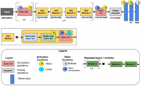
One of the main objectives of this research is to propose an efficient classification model to classify Kannada scene character images. The detailed description of the specifications of the model is shown in Table 1 and the complete flow diagram is depicted in Figure 3. The suggested architecture of AksharaNet is based on inverted DSCs with residuals. Initially two standard separable full 3×3 convolutions are used with 32 and 64 filters having stride 2. These layers are stacked up with four blocks of feature extractors called DSC Modules, with constant expansion factor of 8 applied to the input tensor. Each module/block has three DSC segments, the first 2 segments have residual connections followed by a linear built. Individual segment layer is factorized to a point-wise convolution, a depth-wise convolution [14] with a PReLU [1]. Down sampling is handled with a stride of 2 in the last segment of the block, except at the final DSC module.
A final 1x1 convolution layer with 1024 filters, a global average pooling layer that decreases the spatial resolution to 1, and a dropout layer with 50% removal during training complete the design. Finally, a fully connected layer with a Softmax and a classification layer completes the model. A batch normalization layer is used to bag all convolution layers, but it is not specified in the figures or the table. Except for the first and last modules of the network and the third module of each row, the feature extraction base of the network is made up of 40 convolutional layers organized into 14 modules, all of which have linear connections.
For comparison purposes, we choose the popular Inception v3, MobileNetV2, ResNet-50 and Xception deep CNN models, which are explained in brief below:
InceptionV3: On the ImageNet dataset, Inception v3 is a commonly used image recognition model that has been shown to achieve greater than 78.1 percent accuracy. The model is the accumulation of several theories generated over time by a number of researchers. It is based on Szegedy et al. article [10], "Rethinking the Inception Architecture for Computer Vision." Convolutions, average pooling, max pooling, concats, dropouts, and completely linked layers are among the symmetric and asymmetric building blocks in the model. Batch norm is extended to activation inputs and is used widely in the model. Softmax is used to calculate loss.
MobileNetV2: MobileNetV2 is a convolutional neural network architecture that aims to be mobile-friendly. It is built on an inverted residual system, with residual relations between bottleneck layers. As a source of non-linearity, the intermediate expansion layer filters features with lightweight depth wise convolutions. Overall, MobileNetV2's architecture includes a completely convolutional layer of 32 filters, supplemented by 19 residual bottleneck layers.
Table 1. AksharaNet parameters
|
Layer operation |
Input size |
Kernel size |
Channel count |
Stride |
|
Image |
299×299×3 |
- |
- |
- |
|
Conv1 |
150×150×32 |
3×3 |
32 |
2 |
|
Conv2 |
75×75×64 |
3×3 |
64 |
2 |
|
DSCModule1 |
75×75×192 |
1×1, 3×3 |
192 |
1/1/2 |
|
DSCModule2 |
38×38×256 |
1×1, 3×3 |
256 |
1/1/2 |
|
DSCModule3 |
19×19×512 |
1×1, 3×3 |
512 |
1/1/2 |
|
DSCModule4 |
10×10×768 |
1×1, 3×3 |
768 |
1/1/1 |
|
Conv3 |
10×10×1024 |
1×1 |
1024 |
1 |
|
GAvg Pool |
1×1×1024 |
10×10 |
1024 |
- |
|
FC |
- |
- |
K |
- |
Notes: 1. Each line describes the sequence of layers, 2. DSC Module 1 - 4 refers to the structure as in Figure 3, 3. The kernel size 1×1, 3×3 means pointwise convolution followed by depth wise convolution, 4. The stride 1/1/2 relates to stride of 2 at 3rd convolution module of each block.
Figure 3. Architecture of AksharaNet, a DSC-based classification model
Figure 4. Kannada text classification model using Aksharanet/other CNN models
ResNet-50: ResNet-50 is a 50-layer deep convolutional neural network. You will use the ImageNet database to load a pre-trained version of the network that has been trained on over a million images. The network has been pre-trained to identify images into 1000 object types, including keyboards, mice, pencils, and a variety of animals. As a result, the network has learned a variety of rich feature representations for a variety of images. The network's image input resolution is 224 by 224 pixels.
Xception network: Xception is an extension of the Inception Architecture that uses depthwise Separable Convolutions to replace the regular Inception modules.
Since training all these models requires a lot of computation power, instead of running them out of a datacenter, thanks to Nvidia we can now run them off normal systems using graphical processing units (GPU). Since the computationally intensive part of the neural network is made up of multiple matrix multiplications that run into millions of parameters i.e. weights and biases, we can do all these in parallel (GPU) rather than serially (from a CPU) to speed up operations.
3.2 Implementation
The implementation of the proposed model is split into four stages: Choosing the CNN model, data pre-processing, training and classification and accuracy check. Figure 5 shows the classification model with AksharaNet as the CNN model chosen. The description of each stage is itemized below:
CNN model choice: The CNN models chosen are those that support the current system settings, have properties similar to the proposed model and are presently in use. Along with AksharaNet, InceptionV3, MobileNetV2, Resnet50 and Xception deep CNN models are used to train in Python. At this stage the input size readings are taken from each of these DNN models to transform the image sizes of the dataset accordingly. Also, at the FC layer of the models, the number of filters is replaced to 48-classes in place of 1000. Now, the models are ready to be trained.
Dataset pre-processing: The dataset used here is constrained as per the capacity of the computing system used. Training is done on the vowels and consonants which make 48-classes with 100 images in each class as displayed in Figure 2. The dataset is shuffled and randomly split as train, test and validate sets in 75%, 10% and 15% ratio. These datasets are then scaled up to the size of the DNN model being trained input picture. The photographs are scaled up to 10% horizontally and vertically and randomly converted up to 30 pixels. This data augmentation phase keeps the network from overfitting and memorizing the training images' exact information. While the augmented training set is used to train the network model, the augmented validation set is used to validate the model on a regular basis using training options, and the augmented test set is used for classification.
Training: This segment initializes the hidden parameters for training. The standard settings include execution environment, mini batch size, initial learning rate, momentum, epoch and an optimizer. Here, the models are trained both on the CPU and a single GPU system. A mini-batch size of 35 worked well among other combinations. The initial learning rate is set as 0.01, maximum epoch as 50 and the stochastic gradient descent with momentum (SGDM) is used as an optimizer. The default learning rate drop is at every 10 epoch, a drop of 5 epoch too is examined. The results are tabulated in shown in Figure 7a and Figure 7b. Along with the training options mentioned in the Figure 4, momentum of 0.9 with shuffle at every epoch and L2 regularization for the filters are also applied.
By taking small steps in the direction of the loss function's negative gradient, the SGDM adjusts the network parameters (weights and biases) to minimize the loss function. The additional momentum component aids in the reduction of oscillations that may occur along the steepest descent path to the optimum. For all parameters, the stochastic gradient descent with momentum algorithm uses a single learning rate. The following is the description of this algorithm:
$\theta_{n+1}=\theta_{n}-\propto \nabla E\left(\theta_{n}\right)+\gamma\left(\theta_{n}-\theta_{n-1}\right)$ (1)
where, n denotes the number of steps in the iterative training procedure, $\propto$ is the learning rate, θ the vector of qualified parameters, E(θ) denotes the loss function, and γ is the momentum factor indicating how much the previous step affects the current iteration step.
Classification and accuracy check: The training is carried out using a DNN model with altering hyper parameter values from training options in the augmented training dataset. At every 10th epoch the training is validated with augmented validation. After the iterations are completed, the network is classified with augmented test dataset to make predictions. The accuracy is calculated taking the mean of predictions and test labels, a confusion matrix is generated and sample predictions are displayed. Samples are listed in the Figure 4 where each image is captioned with its class name and percentage accuracy.
Algorithm 1: Training and testing of AksharaNet CNN Model
Initialization
1: Initialize the Keras Libraries and Colab
2: Download the KSIC dataset
3: scale to model image input size
4: Augment images until each class has 1000 samples
5: shuffle and split to Train, Validate and Test sets with labels
Build Neural Network
6: Create a Keras Model for pre-trained Models/AksharaNet
7: Check their input dimensionality to scale the dataset images
8: replace number of classes to 48 in place of 1000 at Fully connected layer
Train, Validate and Test
9: Train the model using augmented train data using mentioned training options (Figure 4)
10: Validate the network for 50 epochs
11: Classify on Test data
12: Calculate test accuracy
The research was conducted in four areas, which are mentioned below:
Performance of all CNN models with and without validation patience using the KSIC dataset on a CPU.
Performance of CNN models and model training time using the KSIC dataset on GPU.
Performance on Early stopping/validation patience (VP).
Performance of CNN models for learning rate drop period.
CNN models are implemented in Python 3.8 using Tensorflow, Keras, OpenCV and sklearnkit. On the hardware side, we trained on a single NVidia RTX GPU and an i7 - 8700 CPU, 8GB RAM, 64-bit OS based system. The dataset consisted of 4800 images with 48-classes that were used for training. AksharaNet and other pre-trained transfer learning models like InceptionV3, MobileNetV2, Resnet50 and Xception are trained and compared for classification. The execution environment with CPU and GPU is tuned to get the best classification performance for the dataset and the proposed models. The results are reported on the augmented training dataset as average training accuracy, on augmented validation dataset as final validation accuracy and on augmented test dataset as testing accuracy.
4.1 Performance of all CNN models with validation patience using the KSIC dataset on a CPU
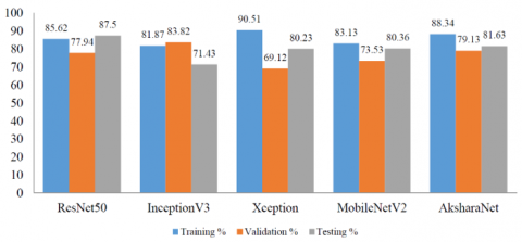
The performance of all the deep neural models is tuned to best case on the Kannada alphabet dataset. Figure 5a compares and shows the execution on a CPU.
The observations are as follows:
From Figure 5a, training accuracy of Xception model is 90.51%, which is good in spite of -5 early stopping/termination. The closure has occurred at 17th epoch (34% of the execution) but with heavy computation time. So using early stopping for this model is good to train and it saves time.
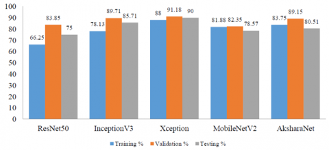
From Figure 5b, Xception model outperforms on validation accuracy with 91.18% with initial learning drop rate of 1e-11 at 15 drops till termination.
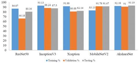
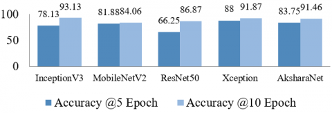
From Figure 5c, InceptionV3 trained the best so far with 93.13% accuracy, while MobileNetV2 gave best validation scores of 91.78% and AksharaNet performed best on testing with 93.19% accuracy.
It is observed that highest values are achieved when lrdf is at a pace of 0.1 for every 10 epoch for 50 max-epoch and without validation patience. Based on these values, the dataset is trained using a GPU next.
Figure 5a. CNN model performance on CPU with early stopping=5 VP and lrdf=5 epoch
Figure 5b. CNN model performance on CPU with normal termination and lrdf=5 epoch
Figure 5c. CNN model performance on CPU with normal termination and lrdf=10 epoch
4.2 Performance of CNN models using the KSIC dataset and GPU
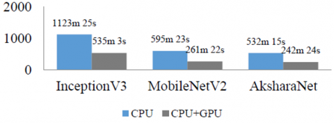
Performance of the models on GPU is shown in Figure 6a and the training time in Figure 6b.
As seen from Figure 6b, GPU takes less than half the time to train the network returning impressive results. From Figure 6a it is observed that InceptionV3 model performs the best with 94.12% validation accuracy, while AksharaNet returns the best testing accuracy. It may be noted that though AksharaNet CPU results are marginally better than GPU for testing, the advantage that GPU offers in terms of half the time for training more than makes up for the marginal increase. Overall, the training time taken by the models in increasing order is AksharaNet, MobileNetV2, Resnet50, InceptionV3 and Xception. AksharaNet in general returns impressive training and validation accuracies and performs best in testing with reduced time frame on the GPU as the model architecture is simple and the number of parameters is lesser in comparison to the other models.
Figure 6a. CNN model performance on GPU
Figure 6b. Model training time on CPU and CPU+GPU
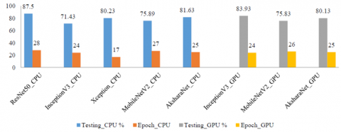
4.3 Early stopping/validation patience (VP) performance
Early stopping entails halting the training automatically by taking benefit from validation data whenever the validation loss stops decreasing. Figure 7a shows the performance of the models for an early stopping VP=5 and Figure 7b without VP on KSIC dataset.
Figure 7a. Model validation patience performance on CPU and GPU with VP=5
Figure 7b. Model validation patience performance on CPU and GPU without VP and Epoch=50
It is observed from Figure 7b that normal training has taken approximately 17-18 drops till completion, Thus VP of 8-9 is ideal for AksharaNet with 50 as max epoch for the considered data. Table 2 mentions the findings based on the various runs. On applying VP, on termination of the training the study is focused on the number of iterations completed, the current learning rate of the network and the training accuracies achieved so far. Early stopping at 50% epoch have accuracies consistent and close to final values. When they read well, the model is trained well; else the current setup combination can be disregarded. In the same context, on reaching termination at 25% epoch, good accuracies provide a scope for improvement while not so good accuracies may or may not improve. Also, for deep models with complex computations early stopping at 25% epoch is ideal (as seen in Xception model in Figure 5a) and 50% epoch for lighter models. Thus, these findings help us to make important decisions, saving a lot of computation time and cost.
Table 2. Early stopping findings based on % Epoch
|
Accuracy |
25% Epoch |
50% Epoch |
|
Bad/average accuracy |
May/may not be accepted |
No scope |
|
Good accuracy |
Scope for improvement |
Acceptable model |
4.4 Performance of CNN models for learning rate drop period
The learning rate parameter is initialized to 0.01 to control the model adaptability with lrdf of 0.1 at each lrdp of the model weights update. Lrdp is examined for a period of every 10 and 5 epochs. Figure 8a (on CPU) and Figure 8b (on GPU) shows performances of the models for the Kannada dataset for both categories of lrdp.
Figure 8a. Model performance for learning rate drop period on CPU
Figure 8b. Model performance for learning rate drop period on GPU
The considerations for drop at every 5 epoch winds up the execution at learning rate of 1e-11 and for drop at every 10 epoch the learning rate is 1e-06. The models exhibit better accuracies with last learning rate up to 1e-06, so decaying of learning rate is ideal at an ample epoch gap extending up to 1e-06. Also, frequent drop calculations add up to overall model computation cost and time.
The proposed work aims to grounds-up curate a dataset in the absence of large-scale Kannada scene character dataset. A dataset with 46,800 Kannada scene character images having 468 classes with 100 images for each class was developed with an objective to use techniques which can help in building a quality dataset which can feed and judge the efficiency of the various models. The dataset is scalable and can be replicated to any size or level through morphing. AksharaNet - a GPU-accelerated deep neural network model with low complexity and computation cost is proposed. Its architecture is tailored for mobile and resource constrained environments providing results with high accuracy and fast computations. The study is investigated on five models and deeper learning allowed us to conclude that on testing data, AksharaNet outperforms MobileNetV2 by 1.5% on CPU and 1.9% on GPU. Training the model with complete 468 classes having 46,800 images on multiple high-end GPUs is expected to increase the performance. The model training time is drastically reduced by 50% when using a GPU compared to only a CPU, with AksharaNet requiring the least time as the model architecture is simple and the number of parameters is lesser in comparison to the other models. Early stopping decisions at 25% epoch and 50% with good and bad accuracies for complex and light models are discussed. Also, useful findings w.r.t. learning rate drop factor and its ideal period for application are enumerated. Overall, AksharaNet returns a robust performance to classify individual characters, which can be extended to words, sentences and numbers as future research. The model can be extended to a spectrum of different model sizes, both depth and width wise hence it can be used for real-time mobile applications like text recognition and translation. The dataset can be augmented or scaled to highest level and also can be used in applications where blur or broken content needs to be classified or replaced.
The authors sincerely acknowledge and thank Mr. Sumit Ranjan and Ms. Vinitha V N for their valuable technical inputs and guidance during the implementation phase of AksharaNet.
[1] Bianco, S., Cadene, R., Celona, L., Napoletano, P. (2018). Benchmark analysis of representative deep neural network architectures. IEEE Access, 6: 64270-64277. https://doi.org/10.1109/ACCESS.2018.2877890
[2] Merati, M., Mahmoudi, S., Chenine, A., Chikh, M.A. (2019). A new triplet convolutional neural network for classification of lesions on mammograms. Revue d’Intelligence Artificielle, 33(3): 213-217. https://doi.org/10.18280/ria.330307
[3] LeCun, Y., Jackel, L.D., Bottou, L., Cortes, C., Denker, J.S., Drucker, H., Guyon, I., Muller, U.A., Sackinger, E., Simard, P., Vapnik, V. (1995). Learning algorithms for classification: A comparison on handwritten digit recognition. Neural networks: The Statistical Mechanics Perspective, World Scientific, 261-276.
[4] Krizhevsky, A., Sutskever, I., Hinton, G.E. (2017). ImageNet classification with deep convolutional neural networks. Communications of the ACM, 60(6): 84-90. https://doi.org/10.1145/3065386
[5] Zeiler, M.D., Fergus, R. (2014). Visualizing and understanding convolutional networks. In: Fleet D., Pajdla T., Schiele B., Tuytelaars T. (eds) Computer Vision – ECCV 2014. ECCV 2014. Lecture Notes in Computer Science, vol 8689. Springer, Cham. https://doi.org/10.1007/978-3-319-10590-1_53
[6] Simonyan, K., Zisserman, A. (2014). Very deep convolutional networks for large-scale image recognition. arXiv preprint arXiv:1409.1556.
[7] Lin, M., Chen, Q., Yan, S. (2013). Network in network. arXiv preprint arXiv:1312.4400.
[8] Szegedy, C., Liu, W., Jia, Y., Sermanet, P., Reed, S., Anguelov, D., Erhan, D., Vanhoucke, V., Rabinovich, A. (2015). Going deeper with convolutions. 2015 IEEE Conference on Computer Vision and Pattern Recognition (CVPR), pp. 1-9. https://doi.org/10.1109/CVPR.2015.7298594
[9] Ioffe, S., Szegedy, C. (2015). Batch normalization: Accelerating deep network training by reducing internal covariate shift. arXiv preprint arXiv:1502.03167.
[10] Szegedy, C., Vanhoucke, V., Ioffe, S., Shlens, J., Wojna, Z. (2016). Rethinking the inception architecture for computer vision. 2016 IEEE Conference on Computer Vision and Pattern Recognition (CVPR), pp. 2818-2826. https://doi.org/10.1109/CVPR.2016.308
[11] Szegedy, C., Ioffe, S., Vanhoucke, V., Alemi, A. (2016). Inception-v4, inception-ResNet and the impact of residual connections on learning. arXiv preprint arXiv:1602.07261.
[12] Sifre, L., Mallat, S. (2014). Rigid-motion scattering for texture classification. arXiv preprint arXiv:1403.1687.
[13] He, K., Zhang, X., Ren, S., Sun, J. (2016). Deep residual learning for image recognition. 2016 IEEE Conference on Computer Vision and Pattern Recognition (CVPR), pp. 770-778. https://doi.org/10.1109/CVPR.2016.90
[14] Chollet, F. (2017). Xception: Deep learning with depthwise separable convolutions. 2017 IEEE Conference on Computer Vision and Pattern Recognition (CVPR), pp. 1800-1807. https://doi.org/10.1109/CVPR.2017.195
[15] Howard, A.G., Zhu, M., Chen, B., Kalenichenko, D., Wang, W., Weyand, T., Adam, H. (2017). Mobilenets: Efficient convolutional neural networks for mobile vision applications. arXiv preprint arXiv:1704.04861.
[16] Sandler, M., Howard, A., Zhu, M., Zhmoginov, A., Chen, L.C. (2018). Mobilenetv2: Inverted residuals and linear bottlenecks. 2018 IEEE/CVF Conference on Computer Vision and Pattern Recognition, pp. 4510-4520. https://doi.org/10.1109/CVPR.2018.00474
[17] Haase, D., Amthor, M. (2020). Rethinking Depthwise Separable Convolutions: How Intra-Kernel Correlations Lead to Improved MobileNets. In Proceedings of the IEEE/CVF Conference on Computer Vision and Pattern Recognition, pp. 14600-14609.
[18] Pal, A., Jaiswal, S., Ghosh, S., Das, N., Nasipuri, M. (2018). SegFast: A faster squeezenet based semantic image segmentation technique using depth-wise separable convolutions. In Proceedings of the 11th Indian Conference on Computer Vision, Graphics and Image Processing, pp. 1-7. https://doi.org/10.1145/3293353.3293406
[19] Tang, D., Jin, M., Wang, Q., Zhou, W., Zhang, J. (2020). Human activity recognition algorithm based on one-dimensional convolutional neural network. Revue d’Intelligence Artificielle, 34(1): 75-80. https://doi.org/10.18280/ria.340110
[20] Mehta, S., Hajishirzi, H., Rastegari, M. (2019). DiCENet: Dimension-wise convolutions for efficient networks. arXiv preprint arXiv:1906.03516.
[21] Kumar, D., Ramakrishnan, A.G. (2012). Recognition of Kannada characters extracted from scene images. In Proceeding of the Workshop on Document Analysis and Recognition, pp. 15-21. https://doi.org/10.1145/2432553.2432557
[22] Aradhya, V.M., Pavithra, M.S., Naveena, C. (2012). A robust multilingual text detection approach based on transforms and wavelet entropy. Procedia Technology, 4: 232-237. https://doi.org/10.1016/j.protcy.2012.05.035
[23] Pavithra, M.S., Aradhya, V.M. (2014). A comprehensive of transforms, Gabor filter and k-means clustering for text detection in images and video. Applied Computing and Informatics, 12(2): 1-15. https://doi.org/10.1016/j.aci.2014.08.001
[24] Yadav, D.P., Kumar, M. (2018). Kannada character recognition in images using histogram of oriented gradients and machine learning. In: Chaudhuri B., Kankanhalli M., Raman B. (eds) Proceedings of 2nd International Conference on Computer Vision & Image Processing. Advances in Intelligent Systems and Computing, vol 704. Springer, Singapore. https://doi.org/10.1007/978-981-10-7898-9_22
[25] Siddiqua, S., Naveena, C., Manvi, S.S. (2019). Recognition of Kannada characters in scene images using neural networks. 2019 Fifth International Conference on Image Information Processing (ICIIP), pp. 146-150. https://doi.org/10.1109/ICIIP47207.2019.8985672
[26] Wu, H., Zou, B., Zhao, Y.Q., Guo, J. (2017). Scene text detection using adaptive color reduction, adjacent character model and hybrid verification strategy. The Visual Computer, 33(1): 113-126. https://doi.org/10.1007/s00371-015-1156-1
[27] Chars74k demo. http://www.ee.surrey.ac.uk/CVSSP/demos/chars74k/, accessed on 12 November 2020.
[28] Siddiqua, S., Naveena, C., Manvi, S.S. (2021). Combined contrast enhanced and wide-baseline technique for text detection in images. Journal of Huazhong University of Science and Technology, 50(4).
[29] Siddiqua, S., Naveena, C., Manvi, S.K. (2017). A combined edge and connected component based approach for Kannada text detection in images. In 2017 International Conference on Recent Advances in Electronics and Communication Technology (ICRAECT), pp. 121-125. https://doi.org/10.1109/ICRAECT.2017.35
[30] Manjunath Aradhya, V.N., Basavaraju, H.T., Guru, D.S. (2019). Decade research on text detection in images/videos: A review. Evolutionary Intelligence, 1-27. https://doi.org/10.1007/s12065-019-00248-z
[31] Basavaraju, H.T., Aradhya, V.M., Guru, D.S. (2019). Text detection through hidden Markov random field and EM-algorithm. In Information systems design and intelligent applications, Springer, Singapore, 19-29. https://doi.org/10.1007/978-981-13-3329-3_3