Siyin Luo | Youjian Gu | Xingxing Yao* | Wei Fan
© 2021 IIETA. This article is published by IIETA and is licensed under the CC BY 4.0 license (http://creativecommons.org/licenses/by/4.0/).
OPEN ACCESS
In view of the fact that a single sentiment classification model may be unstable in classification, this paper attempts to propose a joint neural network and ensemble learning sentiment analysis method. After data preprocessing such as word segmentation on the text, combined with document vectorization method for feature extraction, we then use four basic classifiers including long short-term memory network, convolutional neural network, a serial model combining convolutional neural network and long short-term memory network, and support vector machine to train model, respectively. Finally, the integration is carried out by stacking ensemble learning. The experimental results show that the integrated model significantly improves the accuracy of text sentiment analysis and it can effectively predict the sentiment polarity of the text.
sentiment analysis, document vectorization, long short-term memory network, convolutional neural network, support vector machine, stacking integration
With the rapid development of Internet technology, many network communication platforms have emerged, and users can quickly and conveniently obtain all kinds of required information. The text is the main carrier of information dissemination [1]. The prosperity of information technology has produced a large amount of text data, and then text sentiment analysis has emerged. In general, sentiment analysis means that people use computer technologies such as natural language processing and text analysis to mine and analyze the information in the text to extract the emotional polarity.
In recent years, sentiment analysis has been widely used in marketing, public opinion control, machine translation and other fields. The current text sentiment analysis methods are mainly based on sentiment dictionaries, machine learning, and deep learning. The method based on sentiment dictionary needs to construct sentiment vocabulary manually, and the accuracy of sentiment classification results depends on the perfection of sentiment dictionary [2-5]. Lu and Wu [6] constructed a basic emotion dictionary, a dominant emotion dictionary, a negative word dictionary, and a degree adverb dictionary. They continued to combine the four dictionaries to expand the dictionary, thereby realizing text classification in combination with the sentiment dictionary. Sentiment analysis methods based on machine learning require manual selection of complex features [7], and feature selection determines the final classification results. Pang et al. [8] used simple Bias, maximum entropy and support vector machine (SVM) methods to classify the movie reviews data, and achieved good results. Sentiment analysis methods based on deep learning can automatically extract features and are often used to solve text sentiment analysis problems. Li et al. [9] proposed a hybrid model combining BiLSTM and CNN: the information before and after each word in the text are obtained by BiLSTM, and the CNN feature extraction is adopted for classification. Zhang et al. [10] combined CNN and BiLSTM into a parallel hybrid model CNN_BiLSTM for text classification of Weibo data with an accuracy of 77.44%. Xu et al. [11] proposed the att_C_MGU neural network model, combining the respective advantages of CNN and the minimum gating unit MGU, and fusing the attention mechanism. The classification accuracy rate on IMDB data reached 88.16%.
Single classifiers have limitations and cannot get better classification results. As a means to effectively improve accuracy, ensemble learning has been widely used in many fields. Model integration methods include bagging, boosting, stacking, etc. According to the integrated models, it can be divided into homogeneous integration and heterogeneous integration. The models in homogeneous ensemble learning are of the same type. For example, decision tree ensemble model is full of decision trees, and neural network ensemble model is full of neural networks. The models in heterogeneous ensemble contain different types of individual learners, such as decision trees and neural networks at the same time. For simplicity, the individual learner is also called basic classifier in the sequel. The bagging method and boosting method usually consider homogeneous weak learners, while the stacking ensemble method usually considers heterogeneous weak learners. In particular, Wan and Gao [12] used up to 6 machine learning methods such as random forest to classify sentiment on airline data on Twitter by bagging ensemble method and got a precision of 91.7%. Duan et al. [13] combined the TF-IDF and SVD methods, and then used stacking integrated learning to perform text sentiment analysis on Weibo data, with an accuracy of 81%. Sharma and Jain [14] used n-gram and TF-ID to form different composite feature sets for text vectorization, and then used AdaBoost integration strategy to achieve text sentiment classification.
So far, homogenous ensemble research is still the most common in the field of text sentiment classification. The models in heterogeneous ensemble learning may be difficult to integrate models due to different types. In order to integrate multiple individual learners and obtain better performance than a single individual learner, the performance of the individual learners should not be too bad, and there must be differences between the individual learners. How to generate different models is the key to ensemble learning. Therefore, the basic classifiers in heterogeneous ensemble learning are more diverse, and the differences between models are greater, which effectively improves the classification performance of ensemble models. Now, this paper adopts stacking to achieve heterogeneous integration, including two types of models: neural network and support vector machine.
In this paper, we will use the long short-term memory network (LSTM), convolutional neural network (CNN), a serial model combining convolutional neural network and long short-term memory network (CNN-BiLSTM), support vector machine (SVM) and stacking integrated model realize text sentiment classification. The comparison of the classification results shows that stacking integrated model effectively improves the accuracy of the sentiment classification task of review text. Our main contributions are summarized as follows:
(1) We propose the doc2vec feature extraction method, which can effectively extract sentence features on the basis of acquiring word features. It avoids ignoring the word order of the text and effectively improves the accuracy of text classification.
(2) We propose an ensemble fusion method, using the stacking ensemble method to integrate four common text classification methods (including BiLSTM, CNN, CNN-BiLSTM, SVM), and achieve good classification results.
2.1 Data preprocessing
Due to the diversification of online comment data, there will be many online terms, and even sentences with ambiguous semantics and grammatical errors, which make the text structure complex and increase the difficulty of sentiment analysis. Therefore, it is necessary to perform preprocessing operations such as data cleaning, text length interception, removal of stop words, and Chinese word segmentation on the original text data. For example, data cleaning includes data denoising, removal of meaningless sentences, etc. Text length interception refers to intercepting the same length for each text; removal of stop words means to remove insubstantial words such as modal particles and special symbols in the text; Chinese word segmentation refers to the segmentation of a continuous text sequence into individual words according to certain specifications. Jieba can perform word segmentation at a faster rate while ensuring accuracy, which meets the needs of a large amount of data. Therefore, the data are segmented by Jieba.
Jieba word segmentation has three different word segmentation modes: precise mode, full mode and search engine mode. The precise mode is the most commonly used word segmentation method, that is, trying to cut the sentence most accurately, suitable for text analysis; the full mode can list all possible words in the sentence, but cannot resolve the ambiguity; the search engine mode is suitable for search engines. Here, we use the precise mode of Jieba word segmentation. Jieba comes with a dictionary containing more than 20,000 words, and the text is segmented according to the dictionary. In addition, Jieba word segmentation supports a custom dictionary. In this paper, we analyze the experimental text and add a custom dictionary to include words that are not in the lexicon to ensure a higher accuracy. Examples of the word segmentation results are shown in Figure 1.
Figure 1. Examples of the word segmentation results
2.2 Feature extraction
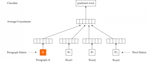
Text feature extraction is one of the core issues to solve text sentiment classification. The key is to extract features that are effective for the classification results from the original data without using all features, avoiding the disaster of dimensionality. Common text feature extraction methods include n-gram, TF-IDF, document frequency and Word2vec [15]. In this paper, the PV-DM algorithm in the Doc2vec [16] model is used to extract text features. Paragraph vectors are added on the basis of Word2vec. Not only can the semantic information of the text be extracted, but also the word order information of the text can be extracted. Once the text reaches the paragraph scale, we can retain word order and context information. The structure of PV-DM is shown in Figure 2.
The Doc2vec text vectorization structure is shown in Figure 2. It connects a paragraph vector with several word vectors in a paragraph, and predicts the next word in a given context. In this framework, each paragraph is mapped to a unique vector, represented by a column in matrix D; each word is mapped into a unique vector Wi, represented by a column in matrix W. The paragraph vector and word vector are averaged or concatenated to predict the next word in the context. In the experiments, we use concatenation as the method to combine the vectors.
Figure 2. The framework of the Doc2vec
For a given sequence of words w1, w2,⋯, wT, the objective function of the word vector model is to maximize the average log probability:
$\frac{\text{1}}{\text{T}}\sum\limits_{t=k}^{T-k}{\log p({{w}_{t}}\text{ }\!\!|\!\!\text{ }{{w}_{t-k}},\cdots ,{{w}_{t+k}})}$ (1)
Prediction is usually done through multiple classification tasks. So we have:
$p({{w}_{t}}|{{w}_{t-k}},\cdots ,{{w}_{t+k}})=\frac{{{e}^{{{y}_{wt}}}}}{\sum\nolimits_{i}{{{e}^{{{y}_{i}}}}}}$ (2)
where, yi represents the unnormalized log probability value of output word i, namely,
${{y}_{i}}=b+Uh{{w}_{t-k}},\cdots ,{{w}_{t+k}};D,W$ (3)
2.3 Basic classifier construction
2.3.1 bidirectional LSTM (BiLSTM)
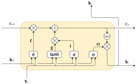
LSTM [17] is widely used in text sentiment analysis tasks, which can give a good sentence semantic representation and model the entire sequence and capture long-term dependencies, solving the defects of gradient disappearance and gradient explosion [18]. LSTM is actually a special RNN that adds a method of carrying information across multiple time steps. LSTM controls the flow of information through three gating mechanisms: the forget gate, the input gate and the output gate. Here, the forget gate controls the selective forgetting of the input at the previous moment; the input gate controls how much the current input is saved to the unit state; the output gate controls the output of the current unit state. The working principle of LSTM is shown in Figure 3.
Figure 3. The framework of the LSTM
As shown in Figure 3, at time t, there are three inputs to LSTM: the input xt of the network at the current time, the output ht-1 of the LSTM at the previous time, and the unit state ct-1 at the previous time; there are two LSTM outputs: the output ht of LSTM at the current time, and the current unit state ct. Note that x, h, and c are all vectors. When the input xt passes through the memory cell unit, it passes through the forget gate, the input gate and the output gate in turn. Some information is selected by the memory unit to be forgotten, and some information is forgotten.
The specific calculation process when input xt passes through the memory unit is as follows:
(1) After the forget gate ft, the forget gate determines what information the memory cell unit discards from the previous state. The calculation formula of the forget gate is:
${{f}_{t}}=\sigma ({{W}_{f}}\cdot [{{h}_{t-1}},{{x}_{t}}]+{{b}_{f}})$ (4)
where, Wf is the weight matrix of the forgetting gate; bf is the bias vector of the forgetting gate; σ is the sigmoid function, the value of the sigmoid function is (0,1), ft is constrained to (0,1) after the operation of the sigmoid function, 1 means “reserve all”, and 0 means “discard all”.
(2) After the input gate it, the input gate determines which information is added to the memory by the memory cell unit, and the calculation formula is:
${{i}_{t}}=\sigma ({{W}_{i}}\cdot [{{h}_{t-1}},{{x}_{t}}]+{{b}_{i}})$ (5)
${{g}_{t}}=tanh({{W}_{g}}\cdot [{{h}_{t-1}},{{x}_{t}}]+{{b}_{g}})$ (6)
where, Wi is the weight matrix of the forgetting gate; bi is the bias vector of the forgetting gate; g represents the new information added to the memory unit; tanh is the hyperbolic tangent function; Wg and bg are the corresponding weight matrix and bias.
(3) After deciding to discard and retain the information, we can update the memory unit, and the formula is:
${{c}_{t}}={{f}_{t}}\odot {{c}_{t-1}}+{{i}_{t}}\odot g$ (7)
where, ct is the updated memory unit, $\odot$ is element multiplication, also called Hadamard product.
(4) Finally, the output gate ot is calculated, and the final output value ht is obtained by ot and ct as follows:
${{o}_{t}}=\sigma ({{W}_{o}}\cdot [{{h}_{t-1}},{{x}_{t}}]+{{b}_{o}})$ (8)
${{h}_{t}}={{o}_{t}}\odot \tanh ({{c}_{t}})$ (9)
where, Wo is the weight matrix of the forgetting gate; bo is the bias vector of the forgetting gate.
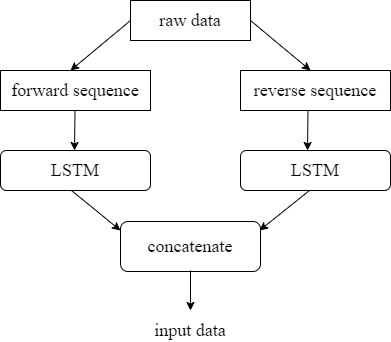
BiLSTM [19] processes the input sequence from the forward and reverse directions. Thus, it can capture features that may be ignored by the one-way LSTM, which obtain more accurate text features and improve accuracy and alleviate the problem of forgetting. The working principle of BiLSTM is shown in Figure 4.
Figure 4. The structure of the BiLSTM
2.3.2 CNN
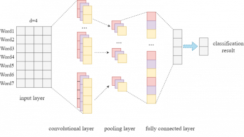
CNN [20] is a feed-forward neural network. Its computing process includes convolution operations. The biggest feature is local perception and parameter sharing, and it performs well in the field of computer vision. In this paper, a one-dimensional CNN is used to extract local subsequences from the sequence, and these subsequences can be recognized anywhere in the input sentence, so that the one-dimensional CNN can learn the local features of different sentences in the entire text and greatly reduce the time complexity of processing text sequences.
Figure 5. The framework of the CNN
As shown in Figure 5, the CNN model consists of four parts: input layer, convolutional layer, pooling layer, and fully connected layer. First of all, the input layer is a matrix representing sentences, the dimension is n×d, that is, there are n words in each sentence, and each word has a d-dimensional word vector representation. The convolution layer uses a convolution kernel K with a width d and a height h to perform convolution operations on the text to obtain corresponding features gi Convolution operation can be computed as:
${{g}_{i}}=f(K\cdot {{X}_{i:i+h-1}}+b)$ (10)
where, Xi:i+h-1 represents the sequence of the words Xi, Xi+1, ⋯, Xi+h-1, and f represents the non-linear activation function Relu. After the convolution operation, an n-h+1 dimensional feature set G can be obtained: G={g1, g2, ⋯, gn-h+1}. We then use the maximum pooling to obtain feature vectors with the same length, and select the maximum value from the feature set to represent the feature value $\hat{G}=\max \{G\}$. Finally, we use the softmax layer of the fully connected layer to output the probability of each category,
${{P}_{i}}=P(y=i|x)=\frac{{{e}^{{{w}_{i}}x+b}}}{\sum\nolimits_{j==1}^{N}{{{e}^{{{w}_{j}}x+b}}}}$ (11)
where, Pi represents the probability of category i, x is the input of the fully connected layer, w is the corresponding weight matrix, b is the bias term, and N is the number of categories.
2.3.3 CNN-BiLSTM
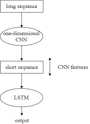
Since CNN can only extract local features of text and is not sensitive to the order of time steps, that is, it cannot well capture the semantics of the text context. LSTM can effectively learn the global features of the text sequences, but its structure is complex, and it takes a long time to process high-dimensional texts [21]. Therefore, we consider the model CNN-BiLSTM that combines CNN and BiLSTM. CNN converts a long input sequence into a short sequence composed of high-level features, and then uses the extracted feature sequence as the input of LSTM, as shown in Figure 6.
2.3.4 SVM
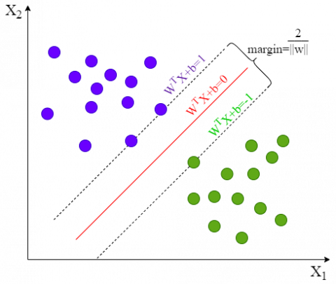
As a representative algorithm in machine learning, SVM is a type of linear classifier based on a supervised learning method. It is widely used in the field of text classification. To use SVM for text classification, firstly, text vectorization and feature extraction must be input into the SVM classifier. For training, the core idea is: for a given linearly separable sample space, establish a hyperplane with a maximum margin to ensure that the distance between the positive and negative samples on both sides of the hyperplane and the hyperplane is maximized [22].
Figure 6. The framework of the CNN-BiLSTM
Figure 7. The structure of the SVM
As shown in Figure 7, the two colored balls in the figure represent two types of samples respectively. The red line in the middle represents the classification plane. The two boundary lines are straight lines drawn along the samples closest to the classification hyperplane in the two types of samples. The distance between them is called the classification margin. To find the hyperplane with the largest classification margin, that is, to transform the problem into a minimum problem with constraints:
$\begin{align} & \underset{w,b}{\mathop{\text{min}}}\,\text{ }\frac{1}{2}\text{ }\!\!|\!\!\text{ }\!\!|\!\!\text{ }w\text{ }\!\!|\!\!\text{ }{{\text{ }\!\!|\!\!\text{ }}^{2}} \\ & \text{s}\text{.t}.\text{ }{{\text{y}}_{\text{i}}}{{w}^{T}}{{x}_{i}}+b\ge 1i=1,2,\ldots ,m. \\ \end{align}$ (12)
2.4 Stacking integration strategy
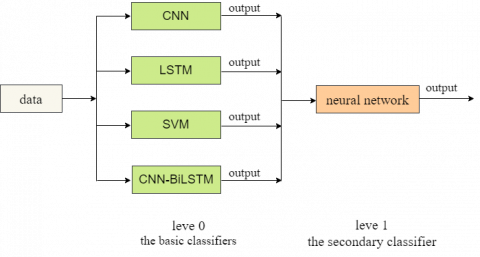
Ensemble learning is to complete the learning task by constructing and combining multiple basic classifiers. Stacking sentiment analysis method is a typical representative of ensemble algorithms [23]. The basic idea of the stacking integration method is: we first use the original data set to train the first-level classifiers; then, we use the outputs of the first-level classifiers as the input feature, and use the corresponding original tag as the new tag to form a new data set to train the second-level classifier.
For example, for the original data set D, we use Dtrain and Dtest to represent the training set and the test set. Given those four learning algorithms above, we then use the t-th learning algorithm to train a first-level classifier $h_{t}^{(\text {train})}$ on Dtrain. For each sample xi in the test set Dtest, let oit be the output result of the learner $h_{t}^{(\text {train})}$ on xi. Then a new data set ${{{D}'}_{{}}}\text{= }\!\!\{\!\!\text{ (}{{o}_{i1}},{{o}_{i2}},{{o}_{i3}},{{o}_{i4}},{{y}_{i}})\}_{i=1}^{m}$ can be generated through them, and the secondary classifier h' will use this data set for training, and the output of the secondary classifier is the final output result.
The basic classifiers used in this paper are CNN, LSTM, SVM and CNN-BiLSTM, and the neural network model is used as the secondary classifier. For the four first-level classifiers, the outputs can be obtained through raw data training. Each output value is a d×1 dimensional vector composed of the sentiment probability value of d sample data. The value is between 0 and 1. Less than 0.5 indicates a negative comment, and greater than or equal to 0.5 indicates a positive comment. And concatenate the four obtained vectors into a d×4 matrix. Finally, the matrix is input into the secondary classifier as an input feature, and a final output of d×1 dimension is obtained. The framework of stacking integration is shown in Figure 8.
Figure 8. The framework of stacking integration
The idea of integrated learning is to ensure the accuracy and differences of individual learners as much as possible. Although the four basic classifiers selected in this paper have different emphasis on data processing, they all maintain a good text classification accuracy and have greater feasibility.
3.1 Experimental environment and Experimental data
The experimental program was compiled in Windows 10, using Python3.6. The deep learning framework is Tensorflow, and the computer runs 32G of memory.
In order to make the model more convincing, the English dataset IMDB and the Chinese dataset Weibo were taken as the corpus. The datasets were divided into training set and test set according to the ratio of 8:2. The detailed data information was shown in Table 1.
Table 1. The dataset
|
Dataset |
Number of comments |
Number of categories |
|
IMDB |
50000 |
2 |
|
|
119988 |
2 |
3.2 Evaluation metrics
Considering that the sentiment polarity of the sentence analyzed in this article is actually a binary classification problem. To verify the effectiveness of the model, accuracy was selected as metrics. The formula is described as follows:
$\operatorname{Accuracy}={{N}_{T}}/N$ (13)
where, NT represents the number of correct sentiment classification predictions, and N represents the total number of samples.
3.3 Model construction
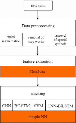
As shown in Figure 9, before application, the original data must receive word segmentation and removal of stop words, and then Doc2vec is used for feature extraction of the data, where the set feature is 600 and the word embedding dimension is 120. After that, four basic classifiers (including CNN, BiLSTM, SVM and CNN-BiLSTM) are used to train data respectively. Finally, we use a simple neural network for stacking integration.
Figure 9. Model overall construction
3.4 Hyperparameter settings
Since the model has different sensitivity to different parameters, the selection of parameters directly affects the final effect of the model.
Table 2. The parameters selection
|
Parameter |
Attribute |
|
Word vector dimension |
120 |
|
Hidden layer size |
128 |
|
batchsize |
128 |
|
Optimization function |
Adam |
|
Dropout rate |
0.2 |
|
Learning rate |
0.1 |
|
Loss function |
Cross entropy |
|
epoch |
20 |
In our experiment, the word embedding dimension was set as 120, the number of hidden layer size as 128, the batchsize as 128. Adam was chosen as the optimizer. To prevent overfitting, a dropout layer is added during training and the initial learning rate was set to 0.1. The cross entropy was defined as the loss function, the experiment is iterated 20 times, and the model parameters were shown in Table 2.
3.5 Model comparison
This subsection compares the ensemble model with the benchmark method of sentiment classification.
GRU: Directly use the GRU model for text sentiment classification [11].
Att-CNN: Introduce the attention mechanism in the CNN classifier [11].
Att-C_MGU: On the basis of att-CNN, the MGU module is introduced to strengthen and optimize the key information of the text features [11].
CNN: Use the CNN model for text sentiment classification [10].
LSTM: Use the LSTM model for text sentiment classification [10].
CNN_BiLSTM: Combine the CNN with BiLSTM into a parallel hybrid model called CNN_BiLSTM [10].
ML-Stacking: Use stacking to integrate multiple machine learning models (including support vector machine, k-Nearest Neighbor, Bayes classifier, etc.) for text sentiment classification [13].
3.6 Results analysis
In order to verify the effect of our model, this section first lists the comparison results of our model and the models above.
Table 3. Classification results of different models on IMDB
|
Model |
IMDB Accuracy (%) |
|
GRU |
86.31 |
|
Att-CNN |
87.25 |
|
Att-C_MGU |
88.16 |
|
Ensemble model in this paper |
97.66 |
Table 4. Classification results of different models on Weibo
|
Model |
Weibo Accuracy (%) |
|
CNN |
74.65 |
|
LSTM |
73.94 |
|
CNN_BiLSTM |
77.44 |
|
ML-Stacking |
81 |
|
Ensemble model in this paper |
94.24 |
As shown in Table 3, the performance of the ensemble model proposed in this paper is significantly better than other benchmark methods. Compared with the other three models, the accuracy of sentiment classification on IMDB data is increased by 9.5%~11.35%, indicating that the ensemble method proposed in this paper has certain feasibility. At the same time, the comparison of the three baseline models shows that the model fused with the attention mechanism has a certain improvement in the accuracy of emotion classification.
As shown in Table 4, the combination of CNN and LSTM is beneficial to improve the accuracy of text classification. Zhang et al. [10] used CNN_BiLSTM and word2vec methods for text classification of Weibo with an accuracy of 77.44%. The ML-Stacking method integrated various machine learning methods and achieved an accuracy of 81%. In this paper, we integrate SVM and neural network, and use Doc2vec for text vectorization. The experimental results show that the accuracy has been significantly improved.
In order to further illustrate the feasibility of the stacking ensemble method used in this article, Table 5 shows the ensemble effect of using three basic classifier under the same experimental environment, and Table 6 shows the integration effect of four basic classifiers.
The comparison of the results in Table 5 and Table 6 shows that the effect of the integration of the four basic classifiers is obviously better than the effect of three basic classifiers. For IMDB data, the result of the integration of the three basic classifiers is not as good as that of a single classifier. For Weibo data, the model after the integration of the three basic classifiers has improved classification accuracy compared to the single model, but it is slightly inferior to the ensemble effect of the four basic classifiers.
Table 5. Integration effect of three basic classifiers
|
Model |
IMDB Accuracy (%) |
Weibo Accuracy (%) |
|
CNN |
96.60 |
86.88 |
|
SVM |
85.94 |
80.27 |
|
CNN-BiLSTM |
97.12 |
86.61 |
|
Ensemble model (three basic classifiers) |
95.66 |
93.97 |
Table 6. Integration effect of four basic classifiers
|
Model |
IMDB Accuracy (%) |
Weibo Accuracy (%) |
|
CNN |
96.60 |
86.88 |
|
BiLSTM |
96.94 |
87.22 |
|
SVM |
85.94 |
80.27 |
|
CNN-BiLSTM |
97.12 |
86.61 |
|
Ensemble model in this paper |
97.66 |
94.24 |
Therefore, we choose four basic classifiers to integrate relatively well. As shown in Table 6, the ensemble model reached 97.66% of English text sentiment classification accuracy, and the accuracy of Chinese text sentiment classification significantly increased to 94.24%. A simple comparison can also be seen that compared with a single classifier, ensemble learning can improve the generalization performance and our model greatly improves the classification accuracy. The results also reflect that on the basis of the high classification accuracy of the basic classifier, the ensemble strategy can only slightly improve the classification accuracy; when the classification accuracy of the basic classifier is relatively low, the ensemble strategy can greatly improve the classification performance.
Compared with using the machine learning model for homogeneous integration, this paper uses the stacking method to integrate SVM and neural network for text sentiment classification, ensuring the differences between different basic classifiers. The results are more comprehensive and convincing, which has certain application prospects. However, the number of basic classifiers is relatively few, and the accuracy can be further improved by increasing the number of basic classifiers; at the same time, the attention mechanism can be integrated into future research to further capture text features.
The sentiment classification method based on neural network and ensemble learning proposed in this paper effectively improves the accuracy of text sentiment classification. This method uses a neural network for a stacking integration strategy to integrate the classification results of multiple basic classifiers (including CNN, LSTM, SVM and CNN-BiLSTM). With the increases in the number of feature features and the word embedding dimension when using the Doc2vec method to process text, the accuracy will rise further. Therefore, the sentiment classification model based on neural network and ensemble learning proposed in this paper is beneficial to improve the accuracy of text classification, and has certain research value in natural language processing.
This work was supported by National Science Foundation of China (Grant No.: 11701434) and Science Foundation of Wuhan Institute of Technology (Grant No.: K201742).
[1] Wang, H., Zhou, C., Li, L. (2019). Design and application of a text clustering algorithm based on parallelized K-means clustering. Revue d'Intelligence Artificielle, 33(6): 453-460. https://doi.org/10.18280/ria.330608
[2] Al-Thubaity, A., Alqahtani, Q., Aljandal, A. (2019). Sentiment lexicon for sentiment analysis of Saudi dialect tweets. Procedia Computer Science, 142: 301-307. https://doi.org/10.1016/j.procs.2018.10.494
[3] Abdi, A., Shamsuddin, S.M., Hasan, S., Piran, Jalil, M.D. (2018). Machine learning-based multi-documents sentiment-oriented summarization using linguistic treatment. Expert Systems with Applications, 109: 66-85. https://doi.org/10.1016/j.eswa.2018.05.010
[4] Zhang, J., Ding, S., Zhang, N. (2018). An overview on probability undirected graphs and their applications in image processing. Neurocomputing, 321: 156-168. https://doi.org/10.1016/j.neucom.2018.07.078
[5] Zhao, X., Ding, S., An, Y., Jia, W. (2018). Asynchronous reinforcement learning algorithms for solving discrete space path planning problems. Applied Intelligence, 48(12): 4889-4904. https://doi.org/1007/s10489-018-1241-z
[6] Lu, K., Wu, J. (2019). Sentiment analysis of film review texts based on sentiment dictionary and SVM. The 2019 3rd International Conference.
[7] Shang, C., Li, M., Feng, S., Jiang, Q., Fan, J. (2013). Feature selection via maximizing global information gain for text classification. Knowledge-Based Systems, 54(4): 298-309. https://doi.org/10.1016/j.knosys.2013.09.019
[8] Pang, B., Lee, L., Vaithyanathan, S. (2002). Thumbs up? sentiment classification using machine learning technique. Proceedings of the ACL-02 Conference on Empirical Methods in Natural Language Processing, 10: 79-86. https://doi.org/10.3115/1118693.1118704
[9] Li, Y., Wang, X., Xu, P. (2018). Chinese text classification model based on deep learning. Future Internet, 10(11): 1-12. https://doi.org/10.3390/fi10110113
[10] Zhang, C., Li, Q., Cheng, X. (2020). Text sentiment classification based on feature fusion. Revue d'Intelligence Artificielle, 34(4): 515-520. https://doi.org/10.18280/ria.340418
[11] Xu, F., Lu, X. (2020). Text sentiment analysis combining convolutional neural network and minimum gating unit attention. Computer Applications and Software, 37(09): 75-80, 125.
[12] Wan, Y., Gao, Q. (2016). An ensemble sentiment classification system of Twitter data for airline services analysis. IEEE International Conference on Data Mining Workshop, pp. 1318-1325. https://doi.org/10.1109/ICDMW.2015.7
[13] Duan, J., Liu, S., Ma, K., Sun, R. (2019). Text sentiment classification method based on ensemble learning. Journal of Jinan University (Natural Science Edition), 33(06): 483-488.
[14] Sharma, S., Jain, A. (2020). Hybrid ensemble learning with feature selection for sentiment classification in social media. International Journal of Information Retrieval Research, 10(2): 40-58. https://doi.org/10.4018/IJIRR.2020040103
[15] Mikolov, T., Sutskever, I., Chen, K., Corrado, G., Dean, J. (2013). Distributed representations of words and phrases and their compositionality. Advances in Neural Information Processing Systems, 26: 3111-3119. https://arxiv.org/abs/1310.4546
[16] Hill, F., Cho, K., Korhonen, A. (2016). Learning distributed representations of sentences from unlabelled data. Proceedings of NAACL-HLT, pp. 1367-1377. https://doi.org/10.18653/v1/N16-1162
[17] Bodapati, J.D., Veeranjaneyulu, N., Shaik, S. (2019). Sentiment analysis from movie reviews using LSTMs. Ingenierie des Systemes d'Information, 24(1): 125-129. https://doi.org/10.18280/ISI.240119
[18] Greff, K., Srivastava, R.K., Koutnik, J., Steunebrink, B.R., Schmidhuber, J. (2016). LSTM: A search space odyssey. IEEE Transactions on Neural Net-work and Learning Systems, 28(10): 2222-2232. https://doi.org/10.1109/TNNLS.2016.2582924
[19] Schuster, M., Paliwal, K.K. (2002). Bidirectional recurrent neural networks. IEEE Transactions on Signal Processing, 45(11): 2673-2681. https://doi.org/10.1109/78.650093
[20] Chirra, V., Reddyuyyala, S., Kishorekolli, V. (2019). Deep CNN: A machine learning approach for driver drowsiness detection based on eye state. Revue d'Intelligence Artificielle, 33(6): 461-466. https://doi.org/10.18280/ria.330609
[21] Neelapu, R., Devi, G.L., Rao, K.S. (2018). Deep learning based conventional neural network architecture for medical image classification. Traitement du Signal, 35(2): 169-182. https://doi.org/10.3166/TS.35.169-182
[22] Dominik, S., Andreas, M., Sven, B. (2010). Evaluation of pooling operations in convolutional architectures for object recognition. International Conference on Artificial Neural Networks, pp. 92-101. https://doi.org/10.1007/978-3-642-15825-4_10
[23] Su, Y., Zhang, Y., Ji, D., Wang, Y., Wu, H. (2012). Ensemble learning for sentiment classification. Chinese Conference on Chinese Lexical Semantics, Springer Berlin Heidelberg. https://doi.org/10.1007/978-3-642-36337-5_10