Praveen Kulkarni* | Rajesh T M
© 2021 IIETA. This article is published by IIETA and is licensed under the CC BY 4.0 license (http://creativecommons.org/licenses/by/4.0/).
OPEN ACCESS
Facial expression recognition assumes a significant function in imparting the feelings and expectations of people. Recognizing facial emotions in an uncontrolled climate is more problematic than in a controlled climate due to progress in hindrance, glare and clamor. This paper, we demonstrate another system for successful facial emotion recognition from ongoing face images. Dissimilar to different strategies which invest a lot of energy by partitioning the picture into squares or entire face pictures; our strategy extricates the discriminative component from notable face areas and afterward consolidates with surface and direction highlights for better portrayal. We also made sub-categories in the main expressions like happy and sad, to identify the level of happiness and sadness and to check whether the person is really happy/sad or acting to be happy/sad. Moreover, we lessen the information measurement by choosing the profoundly discriminative highlights. The proposed system is fit for giving high matching precision rate even within the sight of impediments, light, and commotion. To show the heartiness of the expected structure, it utilized two freely accessible testing dataset. These trial results show that the presentation of the expected structure is superior to current strategies, which demonstrate the impressive capability of consolidating mathematical highlights with appearance-based highlights.
emotion detection, facial expression, happiness and sad expression, Human computer interactions
Robotic face positioning is an interesting and important PC vision problem with numerous professional and rule implementation applications. It is exceptionally simple for people yet difficult to mechanize in electronic applications. Practically speaking, utilizations of programmed face acknowledgment incorporate access control, video-reconnaissance, personality variety, and so that the issue of robotizing the cycle of human face acknowledgment is mind boggling and relies upon numerous boundaries, for example, lighting conditions, facial looks, positions and directions of the human appearances. There has been huge advancement in the ongoing years that incorporates various face acknowledgment and demonstrating frameworks. This calculation is executed in OpenCV. The essential issue to be understood is to actualize a calculation for recognition of countenances in a picture. This can be illuminated effectively by people. In any case, there is an undertaking differentiation to how troublesome it really is to make a PC effectively explain this errand. So as to simple the assignment Viola–Jones restricts themselves to full view frontal upstanding countenances. Short prologues to the establishments of face recognition calculations have examined this paper. For Face recognition we have utilized viola jones calculation and attempt to improve the identification changing the limit estimation of picture and depict the issue of location. Emotion recognition is an element-based methodology in which face math is taken which incorporates face shape and other facial highlights like mouth, eyes and nose and so on the calculation requires 2-D pictures whose limit estimations of forces are contemplated in the estimation of the quantity of the pixels to get the whole face include region. We likewise process the limit box esteem where the face region of interest (ROI) is existing. From distinguished face picture we separate the extricated part of face which are nose, eyes and lip ROI by discontinuous based image segmentation method.
Explores in programmed emotion acknowledgment began during the 1960s. The principal endeavour to mechanized emotion acknowledgment approach consisted of checking the estimations between various facial highlights, [1] for example, the sides of the eyes, the hair lines, openings of nose and so on this endeavour was not excessively much effective. Towards the finish of 1980s, the eigenfaces2 strategies incited more extreme investigates which were utilized to discover a face emotion in a photograph and to think about the pictures of the field has reached up to where the operational utilization of facial emotion acknowledgment on high goal frontal picture was currently practical [2]. The Viola and Jones face identifier is the first historically speaking face recognition structure to give fruitful face identification continuously. It contains three principle thoughts that make it conceivable to run progressively: the necessary picture, classifier learning with Adaboost, and the deliberate course structure [3]. Nonetheless, it delivers a high bogus positive rate and bogus negative when legitimately applied to the information picture [4]. Different exploration commitments have been made to beat these issues, for example, utilizing pre-separating or post-sifting techniques based skin shading channels to give reciprocal data in shading pictures. The creator has been proposed a calculation for face recognition dependent nervous data and shade [5]. In spite of the fact that the outcomes were not precise for all sorts of pictures. As of late, a ton of examination is being done in the vision network to exact emotion finder in genuine work application, specifically, the original work by viola and Jones [6, 7]. The Viola and Jones face locator has become the deformity standard to assemble fruitful face recognition in ascertaining emotions progressively, in any case, it creates a high bogus positive (identifying a face when there is none) and bogus negative rate (not recognizing a face that is available) when straightforwardly applied to the information picture [8]. Different techniques and algorithms for emotional analysis considered from different researchers with accuracy analysed by authors [9].
For detection of face emotions there are many algorithms like Haar Cascades which detects the face and crops the parts of face as the main regions of eyes, mouth and nose. Whereas in region-based identification, the system gives six other sub-regions like nose, right side of cheek area, left side of cheek area, forehead, mouth and eyes this will be based on human cognition knowledge learning.
However, the regions like eyes, mouth, ears and nose will be cropped based on the viola-Jones algorithm, in this system also uses Haar cascading to get the face parts which are important in emotion detection.
Usage of algorithms like adaboost to train and integrate the weak classifiers into stronger classifiers and other classifiers will be cascaded in series so that the face detection accuracy will increase.
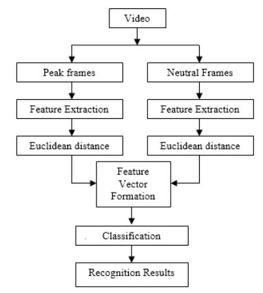
Figure 1. Emotion recognition block diagram
The image will be converted into gray scale which will be effective to describe the face of a human because the human face will have many of the features and it appears there will be enough change of contrast characteristics. Figure 1 gives the entire block diagram for emotion recognition. Due to this Eigenvalues calculation will be time consuming [10]. So here integral graph methodology is used for calculation of Haar like eigen values by this the calculation speed can be improved. The graph method is shown in Figure 2. A(x,y) is the coordinate of graph which is given as the consolidation of every pixel in the topmost left corner.
$A(x, y) i i(x, y)=\sum_{x^{\prime} \leq x, y^{\prime}}^{n} * i\left(x^{\prime}, y^{\prime}\right)$ (1)
From the above equation, ii(x,y) is the elemental image. This original image will be represented as i(x’, y’), the gray values will be gray image information and colour values gives colour image information.
The pixel estimation of a region can be determined by utilizing the basic diagram of the end purposes of the region, as appeared in Figure 2 (b). The pixel estimation of locale D can be determined by
$s(D)=i i(4)+i i(1)-i i(2)-i i(3)$
Figure 2. Integral graph method to calculate eigenvalues
The integral diagram of the organize A(x, y) in a chart is characterized as the amount of the apparent multitude of pixels in its upper left corner.
Here ii(1) speaks to the estimation of pixel from coordinate A, ii(2) shows the pixel estimation of area B+ A, ii(3) shows the pixel estimation of locale C+A, ii(4) shows the pixel estimation of areas D+ C+ B+ A. The rectangular blob represents the eigen values. Considering edges for instance, the estimation of eigenvalue can be communicated by Figure 2 (c). The pixel estimations with respect to A and B coordinates are as follows:
$A s(A)=i i(1)+i i(5)-i i(4)-i i(2)$ (2)
$s(B)=i i(2)+i i(6)-i i(3)-i i(5)$ (3)
As per the definition, the difference between pixel values of region A and region B constitutes the eigen values of rectangular features.
$R=i i(3)-i i(4)+i i(5)-i i(2)-(i i(2)-i i(1))$$-(i i(6)-i i(5))$ (4)
Figure 3. Before normalization after normalization images here
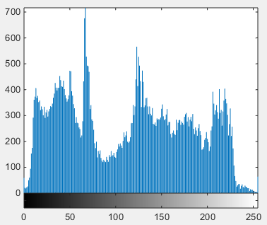
Figure 4. Histogram of the image
Figure 3 shows the image before and after normalization and Figure 4 is the histogram images shown.
In the particular value where the histogram of the image will be constant, the difference between the pixels will be bigger and the entropy value will be biggest [11, 12]. However, dim level adjustment understands the uniform appropriation of picture histogram by which improves differentiation of image and converts the subtleties more clearly, it is helpful for the separation of the facial surface values. For that LBP (Local Binary Pattern) and histogram equalization calculation is utilized.
Level 1 Happiness (Acting to be Happy)
Level 2 Happiness (Appears to be happy)
Level 3 Happiness (Really Happy)
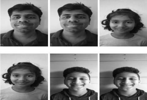
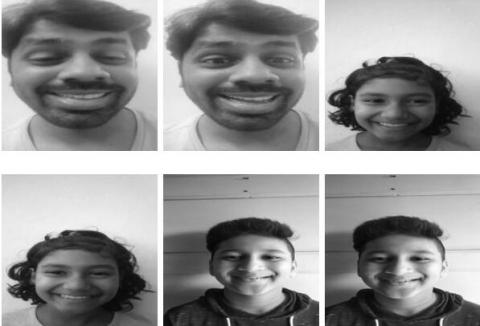
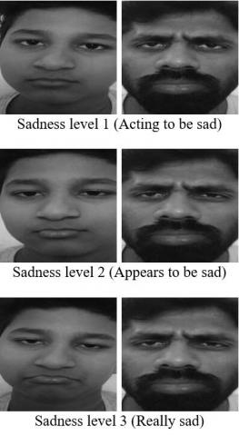
Figure 5. Created dataset for levels of happiness and sad images
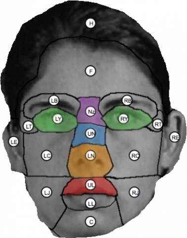
We come up with a bunch of face expressions for marker-based and marker-less frameworks. Previous researchers have considered 12 feature points; in our research we have considered 19 face points to identify the level of emotion in the given emotion. Indeed, we propose a way to deal with separate face points which are really associated with outward appearance. Figure 5 shows the same dataset created for various level of happiness and sad emotion images. Considering more than 7000 images of different 2 to 5 seconds human emotion videos in our experiment initially we considered 19 face points (see Figure 6 and Table 1) where the features are extracted from landmarks set characterized [13] that are normally limited utilizing facial acknowledgment techniques. For testing the measured values we considered a different face image and extraction technique used is a current marker-fewer frame-works for landmark ID and limitation. Their methodology diminishes discovery ambiguities, presents low online computational intricacy and high recognition proficiency beating the other mainstream deformable ongoing models to track and demonstrate non-unbending items framework distinguishes and restricts 66 2D features on face image [14].
Through the dreary perception of facial practices during feeling demeanors, we experimentally pick a subset of 19 facial landmarks that better catch these facial changes among the 66 Face Tracker ones. Utilizing the landmark positions in the picture space, we characterize two classes of highlights: flightiness and direct highlights. These highlights are standardized to the reach [0, 1] to let the element not influenced by individual’s anthropometric attributes conditions [15]. Along these lines, we extricate mathematical relations among landmark positions during enthusiastic articulation for individuals with various nationalities and ages.
Figure 6. Facial landmark points
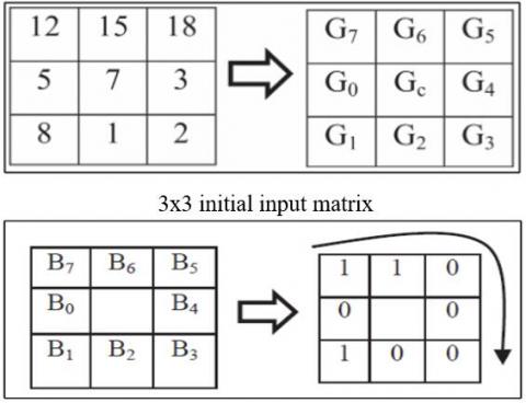
The LBP method functions as follows:
• For each pixel in a picture, a 3 x 3 area is thought of
• The estimation of the middle pixel is contrasted with that of every one of its 8 neighbours.
• If the middle pixel's worth is more noteworthy than that of the neighbour's, a '0' is composed at that neighbour’s area. Something else, a '1' is composed as shown in Figure 7.
• Finally, the 8-bit binary number, beginning from the upper left neighbour, is considered as a decimal number going somewhere in the range of 0 and 255 [16, 17].
Figure 7. Pixel encoding using LBP
• The operator relegates a name to each pixel of an image by thresholding the 3 x 3 neighbourhood of every pixel with the middle pixel esteem.
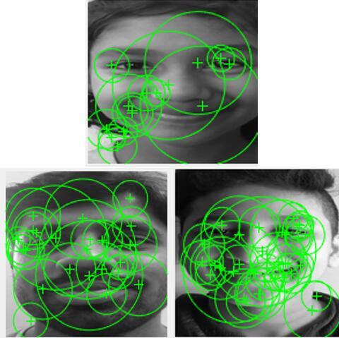
Figure 8. LBP outcome
● LBP functions admirably in various goals and time required for execution is very less as shown in Figure 8 LBP outcome.
● From the redundant neighbourhood points of texture extracted by LBP coordinates will be taken and for those distances will be calculated [18].
● In this work we have taken 19 such data points to calculate the distance as shown in Figure 9 and all the feature values will be tabulated in a csv file for classification.
Figure 9. Distance calculation between the feature points
In this paper we are sub dividing each emotion into a number of sub- categories. If we consider smile as an emotion in that we have divided into levels 1, 2, 3 based on the facial feature points and depending on the distance between eyes, nose and lips.
Table 1. Facial landmark points
|
Number |
Face Landmark |
Class |
|
1 |
Left Eye |
LY |
|
2 |
Right Eye |
RY |
|
3 |
Upper Nose |
UN |
|
4 |
Lower Nose |
LN |
|
5 |
Upper Lip |
UL |
|
6 |
Nasion |
NS |
|
7 |
Lower Lip |
LL |
|
8 |
Right Cheek |
RC |
|
9 |
Left Cheek |
LC |
|
10 |
Right Eyebrow |
RB |
|
11 |
Left Eyebrow |
LB |
|
12 |
Forehead |
F |
|
13 |
Chin |
C |
|
14 |
Right Ear |
RE |
|
15 |
Left Ear |
LE |
|
16 |
Right Jowl |
RJ |
|
17 |
Left Jowl |
LJ |
|
18 |
Right Temple |
RT |
|
19 |
Left Temple |
LT |
Table 2. Different facial feature extraction techniques
|
Techniques Used For Feature Extraction |
Advantages |
Disadvantages |
|
Appearance based |
Number of features are very limited |
It requires very good quality images |
|
Template based |
With template Recognition rate is 100 per cent |
Train & test data must have same set of data |
|
Colour segmentation based |
Matching Colour based |
Fails if colour is discontinuous |
|
Geometry based |
Resolution is low, simple can be done and it is less complex with rate of recognition is 70 per cent |
More features are used |
|
Appearance based |
Number of features are very limited |
It requires very good quality images |
Here face features are controlled by computing the eccentricity of circles developed utilizing explicit facial milestones. Mathematically, the eccentricity quantifies how the oval strays from being round. To consider an oval the eccentricity values must be greater than 0 and it must be less than 1, if the value is equal to 0 then it will be a circle. Forming a model using oval around the mouth by taking feature points like minor and major axis, it will be shown around mouth part eclipse will be drawn with eccentricity greater than 0. The same model will be considered like the eclipse will be drawn around eyes, eyebrows and nose part to get the required features. Along these lines, we utilize the eccentricity to extricate new highlights data and order facial feelings. More in detail, then chose tourist spots for this sort of highlights are 18 more than 19 (see Table 1 and Figure 6), while the complete characterized eccentricity highlights are eight: two in the mouth district, four in the eye area and two in the eyebrow's locale.
Presently, we portray the eccentricity extraction calculation applied to the mouth area [19]. Table 2 represents different feature extraction techniques followed, here we use combination of geometry based with appearance based methods to get better results. As same as the calculation and model created for mouth region these calculations can be further applied for eye and eyebrow regions also. From the below figure taking the eccentricity points an eclipse is drawn and the major axis points are considered as AM and BM. The minor axis points are considered as Um1 and Dm2. Thus, the distance between Um1 with respect to AM and BM is not measured. The best fitting curve will be drawn using the feature points which will be equivalent to the separation of Um1 and with the line AM and BM as shown in Figure 10.
Figure 10. Eccentricity points with drawn eclipse for distance calculation
These are the principle area of interest focuses which we can take as references and dependent on the Euclidean separation figuring strategy the separation between each sub class will be arranged. Here we have considered video inputs which will; be changed over into outlines further and from which we can extricate the information focuses, here we have considered 19 information focuses dependent on the necessity of this work. To recognize faces there are numerous strategies in which Viola Jones end up being the better technique and for face extraction we have utilized a similar strategy and furthermore for eyes, nose and mouth extraction will likewise be finished utilizing a similar technique [20].
As we have considered a video transfer of various degrees of grins, all the edges will be additionally sent for pre-preparing. Pre-handling is one of the primary essentials in picture preparation in the field of PC vision. By this cycle we can remove the significant highlights from the picture to be prepared. This can improve the picture highlights to improve and control the commotion and furthermore repetition of data by applying these means [21, 22].
Starting the initial phase in identification and restriction of face picture to be finished utilizing the accessible classifiers so we can characterize whether the given picture has a face or not.
The acknowledgment module comprises of two stages: (I) highlights extraction to have a test informational index and (ii) grouping. Test informational index was finished by utilizing comparable strides to the preparation information then again; actually it doesn't have the feeling data. Notwithstanding, we utilized the K-Nearest Neighbour calculation (KNN) to characterize an occasion of a test information into a feeling class. Truth is told, KNN order is an incredible grouping technique. The critical thought behind KNN characterization is that comparable perceptions have a place with comparable classes. Hence, one essentially needs to search for the class designator of a specific number of the closest neighbours and summarize their class numbers to relegate a class number to the obscure. Detection of eyes, nose and mouth was done using our own datasets shown in Figure 11.
Figure 11. Eyes, nose and mouth detection using our dataset
Practically speaking, given an occurrence of a test information x, KNN gives the k neighbours closest to the un-named information from the preparation information dependent on the chose separation measure and marks the new example by seeing its closest neighbours using Eq. (5). For our situation, the Euclidean separation is utilized.
$A \mathrm{D}=\sqrt{\sum_{i=1}^{k}(x i-y i)^{2}}$ (5)
where, D is the distance, x and y be the points
The KNN calculation finds the closest preparing examples to the test case. Presently let the k neighbours closest to x b eNk (x) and c(z) be the class name of z. The cardinality of Nk (x) is equivalent to k as shown in Figure 12. At that point the subset of closest neighbours inside class (e) $\in$ the bliss level1, level 2 and level 3.
Figure 12. Feature points for distance calculation
We at that point standardize each Nek (x) by k in order to speak to probabilities of having a place with every feeling class as an incentive somewhere in the range of 0 and 1. Let the lower case nek (x) speak to the standardized worth. The grouping result is characterized as direct blend of the enthusiastic class.
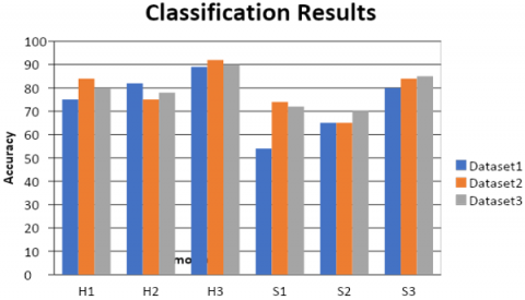
The below graph (Figure 14) shows the classification result of one facial expression of all datasets. The accuracy of happy level 3 is 90%, happy level 2 is 70% and happy level 1 is 80%.
The datset2 is taken as a train informational index. The dataset2 is divided as 80: 20 ratio for testing purpose. The component investigation is performed by utilizing LBP. The surface contrast will be equal to 2. After training model design characterization is carried out. The distance measured between the feature points is the Euclidean distance. For classification is done using KNN (K- nearest neighbour) with k value as 2. The calculation testing is Training/Test. The precision of testing level 1 happiness is 76%, happiness level 2 is 85% and happiness level 3 is 92%. The complete precision rate is 84%.
We take a train informational collection. We have a proportion of 30, 70 test informational collections for arrangement as shown in Figure 13. The element investigation is performed by LBP surface features. The surface distinction is 2. After that design arrangement is performed. The distance measured between the feature points is the Euclidean distance. For classification is done using KNN (K- nearest neighbour) with k value as 2. The classification with the model is carried out. The accuracy of happiness is 80%, the accuracy of happy level 1 is 72%, happy level 2 is 80% and happy level 3 is 85%. The total accuracy rate is 79%.
Figure 13. Training and testing instances neighbour calculation
Figure 14. Result from KNN
In our study different levels of each emotion are detected on the basis of geometrical features of face and calculating the distance between face, nose and eyes. In this research MMI database videos, Japanese Female Facial Expression (JAFFE) Database and some real time expression videos are used. The graph above has shown particular request outcomes of one outward appearance with three levels. Edge computing with LSB and histogram based feature extraction gives better recognition accuracy, the classification algorithm KNN has exhibited most extraordinary precision of 84% at k= 2, where k being k-Nearest Neighbour computation. It is showed up from all the calculation that level 3(real happiness) delight explanations have ideal results of 92% precision over various other expressions. Considering more than 7000 images from different human emotion videos of 2 to 5 seconds in our experiment from international databases, We have taken a train instructive from edge features tabulated in csv file has three levels of euphoria outward appearances of three individuals and we have outright edge shroud test 90 for train educational record reason and 30% periphery cover test for test enlightening list reason and subsequently requested them with better results using LSB method for feature extraction. This whole system can also be automated and used in applications like online video interview etc. to analyze user behavior.
In our research facial expression on frontal face with variations or levels in happiness and sadness are detected and analyzed. Future researches can also consider occlusions, tilt and image contrast for better emotion detection accuracy.
[1] Zhang, Y., Li, Y., Xie, B., Li, X., Zhu, J. (2017). Pupil localization algorithm combining convex area voting and model constraint. Pattern Recognition and Image Analysis, 27(4): 846-854. https://doi.org/10.1134/S1054661817040216
[2] Meng, H., Bianchi-Berthouze, N., Deng, Y., Cheng, J., Cosmas, J.P. (2015). Time-delay neural network for continuous emotional dimension prediction from facial expression sequences. IEEE Transactions on Cybernetics, 46(4): 916-929. https://doi.org/10.1109/TCYB.2015.2418092
[3] Mehmood, R.M., Du, R., Lee, H.J. (2017). Optimal feature selection and deep learning ensembles method for emotion recognition from human brain EEG sensors. IEEE Access, 5: 14797-14806. https://doi.org/10.1109/ACCESS.2017.2724555
[4] Escalera, S., Baró, X., Guyon, I., Escalante, H.J., Tzimiropoulos, G., Valstar, M. (2018). Guest editorial: The computational face. IEEE Transactions on Pattern Analysis and Machine Intelligence, 40(11): 2541-2545. https://doi.org/10.1109/TPAMI.2018.2869610
[5] Feng, X., Zhang, J.P. (2017). Facial Microexpression Recognition: A Survey. ActaAutomaticaSinica, 43(3): 333-348. https://doi.org/10.16383/j.aas.2017.c160398
[6] Özerdem, M.S., Polat, H. (2017). Emotion recognition based on EEG features in movie clips with channel selection. Brain Informatics, 4(4): 241-252. https://doi.org/10.1007/s40708-017-0069-3
[7] Vella, F., Infantino, I., Scardino, G. (2017). Person identification through entropy oriented mean shift clustering of human gaze patterns. Multimedia Tools and Applications, 76(2): 2289-2313. https://doi.org/10.1007/s11042-015-3153-9
[8] Mao, Q., Rao, Q., Yu, Y., Dong, M. (2016). Hierarchical Bayesian theme models for multipose facial expression recognition. IEEE Transactions on Multimedia, 19(4): 861-873. https://doi.org/10.1109/TMM.2016.2629282
[9] Kulkarni, P., Rajesh, T.M. (2020). Analysis on techniques used to recognize and identifying the Human emotions. International Journal of Electrical and Computer Engineering, 10(3): 3307. https://doi.org/10.11591/ijece.v10i3.pp3307-3314
[10] Yu, X., Zhang, S., Yan, Z., Yang, F., Huang, J., Dunbar, N.E. (2014). Is interactional dissynchrony a clue to deception? Insights from automated analysis of nonverbal visual cues. IEEE Transactions on Cybernetics, 45(3): 492-506. https://doi.org/10.1109/TCYB.2014.2329673
[11] Lee, S.H., Plataniotis, K.N., Ro, Y.M. (2014). Intra-class variation reduction using training expression images for sparse representation based facial expression recognition. IEEE Transactions on Affective Computing, 5(3): 340-351. https://doi.org/10.1109/TAFFC.2014.2346515
[12] Ghimire, D., Jeong, S., Lee, J., Park, S.H. (2017). Facial expression recognition based on local region specific features and support vector machines. Multimedia Tools and Applications, 76(6): 7803-7821. https://doi.org/10.1007/s11042-016-3418-y
[13] Kamarol, S.K.A., Jaward, M.H., Kälviäinen, H., Parkkinen, J., Parthiban, R. (2017). Joint facial expression recognition and intensity estimation based on weighted votes of image sequences. Pattern Recognition Letters, 92: 25-32. https://doi.org/10.1016/j.patrec.2017.04.003
[14] Cai, J., Chang, O., Tang, X.L., Xue, C., Wei, C. (2018). Facial expression recognition method based on sparse batch normalization CNN. In 2018 37th Chinese Control Conference (CCC), pp. 9608-9613. https://doi.org/10.23919/ChiCC.2018.8483567
[15] Yang, B., Xiang, X., Xu, D., Wang, X., Yang, X. (2017). 3D palmprint recognition using shape index representation and fragile bits. Multimedia Tools and Applications, 76(14): 15357-15375. https://doi.org/10.1007/s11042-016-3832-1
[16] Kumar, N., Bhargava, D. (2017). A scheme of features fusion for facial expression analysis: A facial action recognition. Journal of Statistics and Management Systems, 20(4): 693-701. https://doi.org/10.1080/09720510.2017.1395189
[17] Takalkar, M., Xu, M., Wu, Q., Chaczko, Z. (2018). A survey: Facial micro-expression recognition. Multimedia Tools and Applications, 77(15): 19301-19325. https://doi.org/10.1007/s11042-017-5317-2
[18] Tzimiropoulos, G., Pantic, M. (2017). Fast algorithms for fitting active appearance models to unconstrained images. International Journal of Computer Vision, 122(1): 17-33. https://doi.org/10.1007/s11263-016-0950-1
[19] Li, J., Zhang, D., Zhang, J., Zhang, J., Li, T., Xia, Y. (2017). Facial expression recognition with faster R-CNN. Procedia Computer Science, 107: 135-140. https://doi.org/10.1016/j.procs.2017.03.069
[20] Xie, S., Hu, H. (2017). Facial expression recognition with FRR-CNN. Electronics Letters, 53(4): 235-237. https://doi.org/10.1049/el.2016.4328
[21] Song, T., Zheng, W., Lu, C., Zong, Y., Zhang, X., Cui, Z. (2019). MPED: A multi-modal physiological emotion database for discrete emotion recognition. IEEE Access, 7: 12177-12191. https://doi.org/10.1109/ACCESS.2019.2891579
[22] Batbaatar, E., Li, M., Ryu, K.H. (2019). Semantic-emotion neural network for emotion recognition from text. IEEE Access, 7: 111866-111878. https://doi.org/10.1109/ACCESS.2019.2934529