Classifying Brain State in Sentence Polarity Exposure: An ANN Model for fMRI Data

The brain is the most complex organ of the human body, responsible for every thought, emotions, feelings, and experiences. It has very complicated neuronal connectivity where each neuron connects with thousands or ten thousand neurons with synapse. The connections and the strength of connection change continuously, and our brain forms millions of new connections every second, which makes it possible to store memories, to learn habits and to shape personalities by reinforcing specific patterns of activities and losing some others. It is found that no two brains are alike, and grey matter in the brain is cell bodies, whereas the white matter is a connection of thread-like structure called axons and dendrites, which connects cell bodies to other neurons. The signals between neurons pass by the release and the capture of neurotransmitter and neuromodulator chemicals like glutamate, acetylcholine, noradrenaline, dopamine, endorphins, and serotonin. The electrochemical signals of neuronal activity are recorded on the scalp using electroencephalography.

In contrast, indirect measurement of neuronal activities is recorded by PET scan and fMRI, which monitor blood flow and CT, and DTI uses the magnetic signature of different tissues. These scanning techniques have revealed which parts of the brain are associated with which functions. Right handed subjects showed right-hemispheric attentional dominance in 95% of cases, and left-hemispheric language dominance in 97% of cases. Left-handed subjects displayed right-hemispheric attentional dominance in 81% of cases, and left-hemispheric language dominance in 74% of cases [1]. Results are in agreement with previous observations ascribing a pre-eminence of the right hemisphere in the processing of negative affective responses in right handed individuals [2]. fMRI study of language processing and its various aspects like syntax, semantics, morphology, etc. in the brain is analyzed for decades.

The processing of syntax in the brain is quietly different from that of –morphology, semantics, etc. [3]. The study and the representation of the syntax (sentence structure) in the brain based on neuroimaging data are enriched in new findings. The research of the syntactic brain grounded on fMRI data can be viewed in five types of sentence arrangements in literature. A) Syntactic violations B) Complex vs. simple sentences C) Sentence vs. word list D) sentences containing pseudo words E) sentences having separate agreements and types.

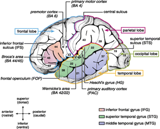
In case of syntactic violation, in which the sentences are syntactically correct but semantically incorrect or having some grammatical error, or spelling error caused increased activation in areas that are involved in syntactic processing due to disruption in agreement checking and structure building which results in more attentive behavior [4]. More superior frontal activity (BA 6, 8) is found for syntactic error compared to any other errors. In grammatical vs. ungrammatical sentences, both types of sentences were presented to the subject, and corresponding fMRI activation was recorded. Syntactically correct and incorrect sentences have different activation patterns and areas of activation in the brain [5]. For complex and simple sentences, the complex sentence involves more syntactic operations, i.e., more reconstruction and canonical word ordering hence activates more area than simple sentences [6]. The enhanced activation in complex sentences lies in Broca’s area (BA 44, 45) extended to BA 47, 6, and 9 [7]. Some additional activation is found in left bilateral superior and middle temporal gyri (BA 21, 22) left angular/supramarginal gyri (BA 39, 40) and cingulate gyrus (BA 23,24,31,32). In the case of sentence vs. word list where a comparison is made between sentence, i.e., syntactic structure and a list of unrelated words, an increased activation is observed for sentence in the anterior part of the temporal lobe, especially temporal pole (BA 38). In addition to this, superior and middle temporal gyri (BA 22 and 21) are also found activated [8]. The comparison of the simple sentence with the pseudoword containing sentences, i.e., sentences that are syntactically correct but consisting of meaningless words (pseudo-words), yielded activation in the posterior superior temporal sulcus (BA 22,41/42). Additionally, anterior superior temporal sulcus (BA 38,22) was also found activated. Figure 1 shows the different brain regions [9] involved in language processing tasks.

However, syntactically and semantically correct sentences are studied by altering its structure and agreements. Lots of research has been done to date, where different forms of sentences are reviewed. Yokoyama et al. [10] have demonstrated the mechanism of case processing in our brain, and the result found shows that the processing of the genitive case activates the left inferior frontal gyrus and posterior part of the middle temporal gyrus more than the nominative case and accusative case for English native speakers.

1.png

Figure 1. Brain anatomy for language processing

The negative sentences are having more syntactic structure than that of affirmative sentences since it contains other syntactic entity for negation [11]. Different negative sentences have diverse representations in the brain, depending on whether these include bipolar predicate or contradictory predicate [12]. Processing of negative sentences is assumed to be a two-step process in which, at first, the affirmative form is processed. Then the negative version of it is represented in the brain, whereas affirmative sentences are directly processed in the brain [13]. The additional syntactic transformation reflects greater cortical activation in the case of negative sentences. Higher activation in the left posterior temporal gyrus and the bilateral parietal brain is observed in negative sentences compared to its affirmative counterpart [14]. In the study of Japanese-English sequential bilingual paradigm with target-probe matching task, a significant activation in left temporal and left pre-central gyrus was observed for negative sentences in English, which is the second language for the participants [15]. Study of action related and abstract sentence polarity sentences have revealed a dynamic mental simulation model of negative sentence processing. Increased activation in the left hemisphere perisylvian and parietal was observed for abstract negative sentences, but a partial deactivation was found in action related negative sentences in left pallidum [16]. For the Danish language, increased activation in the left premotor cortex (BA6) for negative sentences was found [17]. This study reveals that there are three most grave cortical centers for the processing of negative sentences- left premotor cortex (BA6) for sentence structure, bilateral inferior parietal (SMG, BA 40) for semantic processing, and left inferior frontal gyrus dedicated for computation of syntactic complexity. The authors examined the neural correlates of the differences between negative and affirmative sentences using functional magnetic resonance imaging (fMRI), and results found showed enlarged activation in left premotor cortex from negation companionable with rule-governed memory processing and increased activation in the right supramarginal gyrus from affirmation, compatible with semantic processing. In fMRI study [18] of sentences having single and double negation for the German language, it is found that left supplementary motor area (SMA(BA6)) left pars triangularies (BA 45) left pars opercularies (BA44)) and left superior temporal gyrus (STG(BA42)) are functionally associated in the processing of main clause negation. IFG (inferior frontal gyrus) plays the most crucial role in the co-ordination of the cortical areas responsible for language processing and logical reasoning in the interpretation of negative sentences. Kumar et al. [19] have examined fMRI data for activation pattern of the brain in the processing of negative/affirmative sentences of Hindi and found that common cortical region involved in processing includes-bilateral inferior frontal gyrus(IFG), left parietal cortex(BA /40), left fusiform(BA37), bilateral supplementary motor area (SMA (BA6)), bilateral temporal gyrus( BA21) and bilateral occipital area (BA17/18). In addition to this, the study of fMRI data shows that the anterior temporal pole is dedicated to the processing of negative sentences.

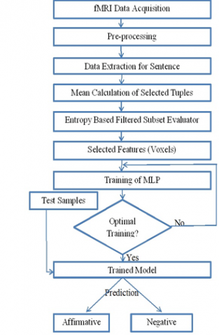
The proposed model utilises correlation based subset evaluator feature selection techniques and multilayer perceptron classification approach in classifying the cognitive state [21] using fMRI data in affirmative and negative sentence processing in the brain. The work flow diagram of the proposed model is represented in Figure 2.

2.png

Figure 2. Work-flow diagram of proposed model

3.1 fMRI data acquisition

T2 weighted -fMRI data were collected from 6 healthy people at the interval of every 500ms. In this experiment a 3.0 T GE Sigma scanner was used, having TE=18ms and a flip angle of 50°. The resulting images captured approximately 5000 voxels per subjects in 8 oblique axial slices in two separate non-contiguous four-slice volumes [22].

3.2 Pre-processing

FIASCO program [23] was used in pre-processing of fMRI images to remove artifacts, i.e., head motion and signal drift, and to correct slice timing. Talairach co-ordinate was used for the normalization of data. 25 anatomical region of interests(ROIs) were selected after pre-processing which includes calcarine sulcus (CALC), left dorsolateral prefrontal cortex (LDLPFC) and right dorsolateral prefrontal cortex(RDLPFC), left inferior parietal lobule (LIPL), left frontal eye fields (LFEF), left intraparietal sulcus (LIPS), right frontal eye fields (RFEF), left inferior frontal gyrus (LIFG), right intraparietal sulcus (RIPS) right inferior parietal lobule(RIPL), supplementary motor areas (SMA), left opercularis (LOPER), right opercularis (ROPER), left and right posterior pre-central sulcus (LPPREC, RPPREC), left and right inferior temporal lobule (LIT, RIT), left temporal (LT) lobe, right temporal lobe, (RT)left and right supramarginal gyrus (LSGA, RSGA), left superior parietal lobule(LSPL), and right superior parietal lobule (RSPL) left and right triangularis (LTRIA, RTRIA).

3.3 Voxel distribution area wise

The data was collected from six persons, and each person has its own identifier id or subject id. For all six persons, their identifiers are following- Subject 04799, Subject 04820, Subject 04847, Subject 05675, Subject 05680, and Subject 05710. The data set comprises of fMRI signal distributed over 24 different anatomical regions of the brain. The analysis of the data set reveals that for the same task, the numbers of voxels involved differ not only anatomical area-wise but subject-wise also. The region-wise distribution of voxel activities is presented in Table 1, which shows the distribution of signal data into different regions of the brain.

3.4 Data extraction and averaging

The data corresponding to the sentence processing is extracted according to the Eq. (1).

The extracted data for classifier training takes the form-

$f: fMRI-sequence (t, t+8) \rightarrow {A Affirmative/Negative sentence}$     (1)

from star plus data-set. The symbol t denotes time. Here 8 sec duration is chosen to capture maximum effective activation signal pattern from data set. 16 images are extracted for 8 sec duration. We calculate the mean of these signals for all voxels. The mean of the extracted data is calculated in accordance with Eq. (2).

$\forall j, j \in \operatorname{column}, \sum_{i=1}^{n} x_{i j} / n$ Where $\mathrm{x}_{\mathrm{ij}}$ is an $\mathrm{i}^{\mathrm{th}}$ row and $j \mathrm{th}$ column entry.     (2)

Table 1. Number of voxels in each anatomical region of the brain

Table 2. Subject wise selected voxels

3.5 Feature selection

For classification, the feature which is highly correlated with the class and having minimal correlation with the other feature is selected considering correlation as goodness measure in feature selection [24]. This feature selection technique works in two steps- first the features are selected relevant to the class and second, iteratively eliminate other features based on the selected feature. Feature which is relevant to the class concept and not redundant to other relevant feature assumed to be good. Correlation measure based on information theoretical concept of entropy for variable x is given by

$H(X)=-\sum_{i=1}^{m} P\left(x_{i}\right) \log _{2}\left(P\left(x_{i}\right)\right)$     (3)

The range of i is from 1 to number of classes (M) The entropy of X after observing the variable Y is represented by

$H(X / Y)=-\sum_{j=1}^{N} P\left(y_{j}\right) \sum_{i=1}^{M} P\left(x_{i} / y_{j}\right) \log _{2}\left(P\left(x_{i} / y_{j}\right)\right)$     (4)

The range of j varies from 1 to N, where N is number of voxels(n).

Where, P(x_i) are the prior probability for all values of X and $P\left(x_{i} / y_{i}\right)$ is the posterior probabilities of X given the values of Y. The information gain is the decrease in entropy of X provided by Y and is given by amount by

$I G(X / Y)=H(X)-H(X / Y)$     (5)

Correlation being biased in favour of features having more value symmetry becomes a measure of correlation between features. Symmetrical uncertainty is represented as

$S U(X, Y)=2\left[\frac{I G(X / Y)}{H(X)+H(Y)}\right]$     (6)

Taking symmetrical uncertainty as goodness measure, relevant features are selected. The range of SU lies between 0 and 1. After finding the values of SU for all features we have selected the top dominating voxels based on the threshold value of SU. For data set S containing N features and C classes, symmetrical uncertainty is denoted as SU_ic for correlation between F_i and class C.

Then

$\forall F_{i} \in S, 1 \leq i \leq N, S U_{i} \geq \delta,(\delta \rightarrow \text { threshold })$

The highly correlated features which are obtained by minimizing the redundancy are summed up in in Table 2. The procedure recursively eliminates the irrelevant feature from the fMRI data and selects only those which are correlated.

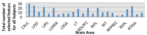
The region wise distribution of selected features in different bran regions is shown in the Table 3. Region-wise number of voxel selected in the determination of sentence classification from all six subjects when summed up category wise becomes -CALC(28), LDLPFC(24), LFEF(10), LIPL(21), LIPS(6), LIT(19), LOPER(5), LPPREC(7), LSGA(7), LSPL(11), LT(17), LTRIA(7), RDLPFC(19), RFEF(6), RIPL(19), RIPS(9), RIT(10), ROPER(8), RPPREC(2), RSGA(4), RSPL(16), RT(23), RTRIA(5), SMA(8).

Table 3. Region-wise distribution of selected feature

From this discussion it’s clear that the most contributing voxels comes from region CALC and LDLPFC. Figure 3 represents the total number of features selected from different region of brain for all subjects.

3.png

Figure 3. Region-wise total number of selected features from all subject

3.6 Classification using multilayer perceptron

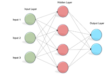
A multilayer perceptron (MLP) [25, 26] is a class of feed forward artificial neural network. MLP consists of at least three layers of nodes: an input layer, a hidden layer and an output layer. Figure 4 represents the architecture of MLP. Except for the input nodes, each node that uses a nonlinear activation function. MLP utilizes a supervised learning technique called back propagation [27] for training:

4.png

Figure 4. Multilayer perceptron

Single-hidden-layer MLP function can be seen as f: R^D→R^L, where the size of input vector x is D, and the size of the output vector f(x) is L,

The matrix notation is given as

$f(x)=G\left(b^{(2)}+W^{(2)}\left(s\left(b^{(1)}+W^{(1)} x\right)\right)\right)$     (7)

With b⁽¹⁾, b⁽²⁾ are bias vectors; W⁽¹⁾, W⁽²⁾ are weight matrices, and, G and s are activation functions.

The hidden layer is

$h(x)=\phi(x)=s\left(b^{(1)}+W^{(1)} x\right)$     (8)

where, $W^{(1)} \in R^{D * D_{h}}$ is the weight matrix connecting the input vector to the hidden layer. Each column Wi⁽¹⁾ represents the weights from the input units to the i^th hidden unit.

The choice for S is given by

$\tanh (a)=\left(e^{a}-e^{-a}\right) /\left(e^{a}+e^{-a}\right)$     (9)

The output vector is then obtained as:

$o(x)=G\left(b^{(2)}+W^{(2)} h(x)\right)$     (10)

The selected feature vectors are fed to the classifier. The classifier is trained to classify the brain state in the processing of affirmative sentences and negative sentences with the assumption that- a) fMRI data has sufficient information to find out the state of the brain corresponding to specific sentence type b) Machine learning algorithm is well efficient to learn the particular temporal pattern to distinguish between the processing of negative vs. affirmative sentences. MLP classification technique is applied to classify the selected feature vectors. In this paper, gradient descent method is used for updating weights and bias during the training of the MLP. Bias nodes are added to increase the flexibility of the model to fit the data by allowing the activation function to be shifted to the left or right. At the beginning, network is initialised with small random weights and then gradient descent is used to tune the weighs into optimized values. Initially, the value of bias is set to 0 and later gradient descent optimizer is used to tune the bias. After the training the model can detect the brain state corresponding to affirmative or negative sentences.

 The performance of a classifier is judged upon the number of wrongly classified instances, i.e., the error rate or misclassification. The goal of the classification model is the determination of its ability to correctly classifying or predicting the class of instances. The confusion matrix explores the error and correctly classified test data in terms of true positive, false positive, etc. The number of correct and incorrect predictions is displayed by the confusion matrix in Table 4. The column entries represent the predicted class value, and rows display the actual class values.

The metrics used in the study are given below-

•TP Rate stands for the rate of true positives, i.e., correctly classified instances as a given class.

•FP Rate means the rate of false positives, i.e., falsely classified instances as a given class.

•Precision: the proportion of instances that are true of a class divided by the total cases classified as that class

•Recall: the proportion of instances classified as a given class divided by the actual total in that class (equivalent to TP rate)

•F-Measure is the harmonic mean of recall and precision and defined as 2 * Precision * Recall / (Precision + Recall)

•MCC is used in machine learning as a measure of the quality of binary (two-class) classifications. It takes into account true and false positives and negatives and is generally regarded as a balanced measure which can be used even if the classes are of very different sizes

•ROC (Receiver Operating Characteristics) area gives an idea of how the classifiers are performing in general.

The model is trained on the selected feature vector data set and tested on the ten-fold cross-validation approach. The accuracy of the result is good enough and can detect sentence polarity with more than 93% accuracy. Table 5 shows the subject wise accuracy result of the sentence polarity task. The average of overall performance analysis in the sentence polarity task is represented in Figure 5, where the performance metric is as following- TP Rate: 0.933333, FP Rate: 0.066667, Precision: 0.940167, Recall: 0.933333, F-Measure: 0.933, ROC Area: 0.980167, Accuracy: 0.933333. The result obtained is quite appreciable as the average classification accuracy of the brain state in the sentence polarity task is more than 93%.

Table 4. Confusion matrix

3.7 Comparative analysis

Behroozi et al. [28] have classified the voxel from the RDLPFC area and achieved an accuracy of almost 75% for all the subjects on the same data set. They have used F-score based feature selection and SVM classification techniques in the classification of selected attributes. In our approach, we have scored more than 93% accuracy in polarity detection. 

Doborjeh et al. [29] have studied the neural activity of affirmative and negative sentences and using NeuCube [30] on the same data set. With proper training after implementing classifiers to classify the neural activity pattern of negative and affirmative sentences in the brain, this model was able to recognize the sentence based on their polarity up to 90% accuracy.

From the above studies, it is clear that our result is evident and has much better classification accuracy than previous approaches. Comparing the classification accuracy of the proposed model with the above-mentioned approaches, the result obtained in the proposed model is significantly higher. Figure 6 shows the comparative analysis of the accuracy of the proposed model with the above-mentioned approaches.

This study is an attempt to recite the state of the brain based on fMRI data acquired when the subjects are indulged in reading two types of sentences i.e. affirmative or negative sentence. Brain processes affirmative and negative sentences differently and the activation produced in the brain is not alike for both types of sentences.

Table 5. The classification result

5.png

Figure 5. Average of results for all subjects

6.png

Figure 6. Comparative accuracies of recent works on the same data-set