Nagadevi Darapureddy* | Nagaprakash Karatapu | Tirumala Krishna Battula
© 2020 IIETA. This article is published by IIETA and is licensed under the CC BY 4.0 license (http://creativecommons.org/licenses/by/4.0/).
OPEN ACCESS
This paper examines a hybrid pattern i.e. Local derivative Vector pattern and comparasion of this pattern over other different patterns for content-based medical image retrieval. In recent years Pattern-based texture analysis has significant popularity for a variety of tasks like image recognition, image and texture classification, and object detection, etc. In literature, different patterns exist for texture analysis. This paper aims at forming a hybrid pattern compared in terms of precision, recall and F1-score with different patterns like Local Binary Pattern (LBP), Local Derivative Pattern (LDP), Completed Local Binary Pattern (CLBP), Local Tetra Pattern (LTrP), Local Vector Pattern (LVP) and Local Anisotropic Pattern (LAP) which were applied on medical images for image retrieval. The proposed method is evaluated on different modalities of medical images. The results of the proposed hybrid pattern show biased performance compared to the state-of-the-art. So this can further extended with other pattern to form a hybrid pattern.
Local Binary Pattern (LBP), Local Derivative Pattern (LDP), Completed Local Binary Pattern (CLBP), Local Tetra Pattern (LTrP), Local Vector Pattern (LVP), Local Anisotropic Pattern (LAP)
Current research work Content Based Medical Image Retrieval (CBMIR) attempts to capture and utilize the semantics of the image to achieve more reliable retrieval which is a challenging task. Image database management retrieval has continued to be an active research area after the 1970s [1]. In 1992, the word, Content-based image retrieval (CBIR) was originated, used by T. Kato to explain experiments into automatic retrieval of images from a database, based on the shapes and colors present. CBIR systems derive characteristics from the raw images themselves and determine an association (similarity or dissimilarity) measure among a query image and database images. CBIR is growing very familiar because of the high demand for searching image databases of ever-growing size. As accuracy and speed are essential, we need to generate a system for retrieving images of both efficient and effective. Textures [2, 3] are defined based on image features extracted and analysis methods. Though texture, is thought of as reconstructed patterns of pixels over a spatial domain, concerning the addition of noise to the patterns and their repetition frequencies results in textures that can appear to be random and unstructured. Image texture, in computer vision, defined as a description of image structure, granularity, randomness, linearity, and roughness. Image feature is considered for describing the innate surface properties of a selected object and its relationship with the surrounding regions [4]. Texture characteristics are remarkable in pattern recognition, image retrieval tasks, as they are present in many real images. Drawbacks of texture-based image retrieval systems are computation complexity and retrieval accuracy. Considering a wide range of different situations, local descriptors or local patterns are advantageous above conventional global features as they are invariant to image scale and rotation and provide robust matching [5]. We will exhibit and review the most popular and recent algorithms with their variants [6], as the research attention in the field of medical images have adapted to use these local features.
The remainder of this paper is organized as: Section 2 introduces about related work, section 3 describes the methodology implemented, section 4 gives the results obtained and section 5 describes the conclusion and future scope.
2.1 Local Binary Pattern (LBP)
LBP [7] is one type of visual descriptor which is used for image retrieval. This pattern got reputation from 2002 for its simplicity in computations and performance with its variants. LBP computes the local representation of texture. While computing LBP two parameters to be considered are ‘P’ pixels which control the quantization of angular space, ‘R’ radius determines the spatial resolution. LBP is robust as it is invariant against any monotonic transformation of the grayscale. LBP descriptor generates binary code by comparing P neighbor pixel with the center pixel. Figure 1 shows different pixel values with different radius.
LBP pattern is formed by taking a particular grey pixel and compared with center pixel by using Eq. (1)
$\begin{aligned}
&\mathrm{LBP}=1 \text { if } \mathrm{g}_{\mathrm{p}} \geq \mathrm{g}_{\mathrm{S}}\\
&=0 \text { else }
\end{aligned}$ (1)
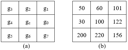
where, gp, the pixel value of P neighbors and gc, grey value of a center pixel. Below example shows how calculate the binary pattern with 8 neighborhood and radius one. Figure 2 and Figure 3 shows the example of how to calculate LBP of 3x3 grey pixels.
Figure 1. Examples of circular neighborhoods with different P and R values
Example:
Figure 2. Neighborhood representation of (a) grayscale image (b) grayscale values
Figure 3. (a) Thresholded on center value (b) binary weights (c) convolved values
$L B P_{P . R} \quad=\sum_{p=0}^{p-1} s\left(g_{p}-g_{c} c\right) 2^{p}$ (2)
$\begin{array}{c}
L B P \text { Code }=1+2+32+64+128=227 \\
\text { LBP pattern }=11100011
\end{array}$ (3)
Singh [8] developed the completed LBP (CLBP) proposal, as LBP has a restraint that it loses the global spatial information. The CLBP denotes the local region by local difference sign-magnitude transforms (LDSMT) and its center pixel. The image gray level described by the center pixels that are transformed into a binary code referred to as CLBP-center (CLBP_C) by global thresholding. Vital development attained for rotation invariant texture classification when CLBP_C united with two operators, namely CLBP-sign (CLBP_S) and CLBP-magnitude (CLBP_M), into hybrid distributions.
2.2 Complete Local Binary Pattern (CLBP)
LBP pattern considers only signs of local differences i.e. difference of every pixel with its neighbors whereas CLBP considers both sign and magnitude of local difference as well as original center grey level value. CLBP is a combination of three values. One is used to code the sign value of local differences given as CLBP_S same as LBP. The other one is used to code the magnitude value of local differences given as CLBP_M. Original center grey level value is given as CLBP.
Sign component is given as:
$S_{p}=S\left(g_{p}-g_{c}\right)$ (4)
where, gc indicate gray value of center pixel and gp (p=0… p-1) gray value of neighbor pixel on a circle of radius R and P is number of the neighbors.
Magnitude component is given as:
$M_{p}=\left|g_{p}-g_{c}\right|$ (5)
CLBP_S is given as:
$\begin{aligned}
C L B P_{-} S_{P, R} &=\sum_{P=0}^{P-1} 2^{P} S\left(g_{p}-g_{c}\right), \\
S_{P} &=\left\{\begin{array}{l}
1, g_{p} \geq g_{c} \\
0, g_{p}<g_{c}
\end{array}\right.
\end{aligned}$ (6)
CLBP_M is given as:
$\begin{array}{l}
C L B P_{M P, R}=\sum_{P=0}^{P-1} 2^{P} t\left(m_{p}, c\right) \\
t\left(m_{p}, c\right)=\left\{\begin{array}{l}
1,\left|g_{p}-g_{c}\right| \geq c \\
0,\left|g_{p}-g_{c}\right|<c
\end{array}\right.
\end{array}$ (7)
CLBP_C is given as:
$C L B P_{C_{P, R}}=t\left(g_{c}, c_{I}\right)$ (8)
where, gc gives gray value of center pixel and cI gives an average gray value of the whole image. Below example shows how calculate the CLBP pattern with 8 neighborhood and radius one. Figure 4 and Figure 5 shows the example of calculation of CLBP pattern.
Example:
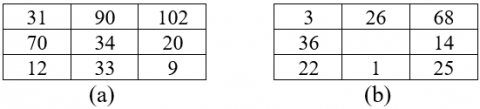
Figure 4. (a) Original image (b) Local difference
Figure 5. (a) CLBP_S =01101000 (b) Assume threshold = 29, CLBP_M=01101000
2.3 Local Derivative Pattern (LDP)
Zhang [6] have introduced local derivative patterns (LDP) approach and extended the LBP to the nth order LDP’s as LBP is a non-directional first-order pattern extracted from first-order derivatives. LDP encodes spatial relationship in a local region by higher order derivative. It is an (n-1)th order derivative which extracts more information than first order binary pattern.
The first order derivatives along 0°, 45°, 90°, 135° directions considering Figure 2 grey scale image given as
$I_{0^{0}}^{\prime}\left(g_{c}\right)=I\left(g_{c}\right)-I\left(g_{0}\right)$ (9)
$I_{45^{\circ}}^{\prime}\left(g_{c}\right)=I\left(g_{c}\right)-I\left(g_{1}\right)$ (10)
$I_{90^{\circ}}^{\prime}\left(g_{c}\right)=I\left(g_{c}\right)-I\left(g_{2}\right)$ (11)
$I_{135^{\circ}}^{\prime}\left(g_{c}\right)=I\left(g_{c}\right)-I\left(g_{3}\right)$ (12)
The second order directional LDP given as
$\begin{array}{c}
L D P_{\alpha}^{2}(g)=
\left\{f\left(I_{\alpha}^{\prime}\left(g_{c}\right), I_{\alpha}^{\prime}\left(g_{0}\right)\right), f\left(I_{\alpha}^{\prime}\left(g_{c}\right), I_{\alpha}^{\prime}\left(g_{1}\right)\right), \ldots, f\left(I_{\alpha}^{\prime}\left(g_{c}\right), I_{\alpha}^{\prime}\left(g_{7}\right)\right)\right\}
\end{array}$ (13)
$\begin{array}{l}
f\left(I_{\alpha}^{\prime}\left(g_{c}\right), I_{\alpha}^{\prime}\left(g_{i}\right)\right) \\
=\left\{\begin{array}{ll}
0, & \text { if }\left(I_{\alpha}^{\prime}\left(g_{c}\right) . I_{\alpha}^{\prime}\left(g_{i}\right)>0\right. \\
1, & \text { if }\left(I_{\alpha}^{\prime}\left(g_{c}\right) \cdot I_{\alpha}^{\prime}\left(g_{i}\right) \leq 0\right.
\end{array} i=0,1, \ldots 7\right.
\end{array}$ (14)
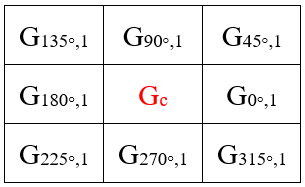
The second order derivative pattern is defined as concatenation of four 8-bit directional LDPs given Figure 6 with primitive patterns.
$L D P^{2}(g)=L D P_{\alpha}^{2}(g)\left\{\alpha=0^{\circ}, 45^{\circ}, 90^{\circ}, 135^{\circ}\right\}$
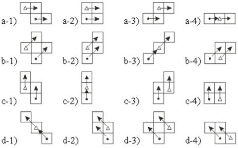
Figure 6. Primitive patterns used in LDP. (a) $\alpha=0^{\circ}$ ref 1=◦, ref2=∆; (b) $\alpha=45^{\circ}$ ref 1=◦, ref 2=∆; (c) $\alpha=90^{\circ}$ ref 1=◦, ref 2=∆; (d) $\alpha=135^{\circ}$ ref 1=◦, ref 2=∆
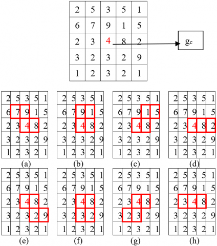
Below example shows how calculate second order LDP pattern with primitive patterns (template) on a patch of grey scale image.
Example:
Figure 7. a) Template (a-1); ref 1=gc; bit obtained=0 b) Template (a-2); ref 1=gc; bit obtained=1 c) Template (a-3); ref 1=gc; bit obtained=0 d) Template (a-4); ref 1=gc; bit obtained=1 e) Template (a-1); ref 2=gc; bit obtained=0 f) Template (a-2); ref 2=gc; bit obtained=1 g) Template (a-3); ref 2=gc; bit obtained=0 h) Template (a-4); ref 2=gc; bit obtained=0
The second order derivative pattern at α=0° using primitive pattern a-1 to a-4
$L D P_{0^{\circ}}^{2}\left(g_{c}\right)=01010100$ (15)
Similarly the second order derivative pattern at α=45° using primitive pattern b-1 to b-4
$L D P_{45^{\circ}}^{2}\left(g_{c}\right)=00101111$ (16)
Similarly the second order derivative pattern at α=90° using primitive pattern c-1 to c-4
$L D P_{90^{\circ}}^{2}\left(g_{c}\right)=11010000$ (17)
Similarly the second order derivative pattern at α=135° using primitive pattern d-1 to d-4
$L D P_{135^{\circ}}^{2}\left(g_{c}\right)=11000110$ (18)
LBP, LDP, with their variants are sensitive to illumination, pose, and facial expression which occur in unconstrained natural images extract the information based upon the distribution of edges that are formed by only two directions (i.e. positive or negative). Murala et al. [9] proposed a successful algorithm based on four directions to improve the performance, namely the local tetra patterns (LTrPs) and significantly used in the CBIR domain.
2.4 Local Tetra Pattern (LTrP)
LTrP is calculated by first-order derivatives of a center pixel along 0° and 90° i.e. vertical and horizontal directions which are calculated by subtracting its gray value of the center pixel with its horizontal and vertical gray values. Let gc denote the center pixel of image I, and gh and gv, the horizontal and vertical neighborhoods respectively of gc considering Figure 2 grey scale image.
The LTrP pattern with first-order derivative at gc can be given as
$I_{0^{\circ}}^{1}\left(g_{c}\right)=I\left(g_{h}\right)-I\left(g_{c}\right)$ (19)
$I_{90^{\circ}}^{1}\left(g_{c}\right)=I\left(g_{v}\right)-I\left(g_{c}\right)$ (20)
And center pixel direction can be given as
$I_{\text {Dir. }}^{1}\left(g_{c}\right)=\left\{\begin{array}{ll}
1 . & I_{0}^{1}\left(g_{c}\right) \geq 0 \text { and } I_{90^{\circ}}^{1}\left(g_{c}\right) \geq 0 \\
2 . & I_{0^{\circ}}^{1}\left(g_{c}\right)<0 \text { and } I_{90^{\circ}}^{1}\left(g_{c}\right) \geq 0 \\
3 . & I_{0}^{1}\left(g_{c}\right)<0 \text { and } I_{90^{\circ}}^{1}\left(g_{c}\right)<0 \\
4 . & I_{0^{\circ}}^{1}\left(g_{c}\right) \geq 0 \text { and } I_{90^{\circ}}^{1}\left(g_{c}\right)<0
\end{array}\right.$ (21)
The second order LtrP is defined
$\begin{aligned}
L T r P^{2}\left(g_{c}\right)=\{& f_{3}\left(I_{D i r}^{1}\left(g_{c}\right) \cdot I_{D i r .}^{1}\left(g_{1}\right)\right), f_{3}\left(I_{D i r .}^{1}\left(g_{c}\right) \cdot I_{D i r .}^{1}\left(g_{2}\right)\right), \\
&\left.\ldots, f_{3}\left(I_{\text {Dir. }}^{1}\left(g_{c}\right) \cdot I_{\text {Dir. }}^{1}\left(g_{P}\right)\right)\right\}\left.\right|_{P=8}
\end{aligned}$ (22)
$\begin{array}{l}
f_{3}\left(I_{\text {Dir. }}^{1}\left(g_{c}\right) \cdot I_{\text {Dir. }}^{1}\left(g_{P}\right)\right) \\
=\left\{\begin{array}{cc}
0, & I_{\text {Dir. }}^{1}\left(g_{c}\right)=I_{\text {Dir. }}^{1}\left(g_{P}\right) \\
I_{\text {Dir. }}^{1}\left(g_{P}\right) & \text { else }
\end{array}\right.
\end{array}$ (23)
$\begin{array}{l}
f_{3}\left(I_{\text {Dir. }}^{1}\left(g_{c}\right) \cdot I_{\text {Dir. }}^{1}\left(g_{P}\right)\right) \\
=\left\{\begin{array}{lr}
0, & I_{\text {Dir. }}^{1}\left(g_{c}\right)=I_{\text {Dir. }}^{1}\left(g_{P}\right) \\
I_{\text {Dir. }}^{1}\left(g_{P}\right) & \text { else }
\end{array}\right.
\end{array}$ (24)
From Eqns. (23) and (24), an 8 bit tetra pattern for each centre pixel is obtained and then it separates all patterns into four parts depending on the direction of center pixel. Finally, three patterns from the tetra patterns are achieved.
Let the direction of center pixel obtained from Eq. (23) be "1" then LTrP2 can be defined by dividing it into three binary patterns as shown in Eq. (25) as follows
$\begin{array}{l}
\left.L T r P^{2}\right|_{\text {Direction }}=2,3,4 \\
=\left.\sum_{\mathrm{p}-1}^{P} 2^{(p-1)} \mathrm{X} f_{4}\left(\operatorname{LTr} \mathrm{P}^{2}\left(g_{c}\right)\right)\right|_{\text {Direction }=2,3,4}
\end{array}$ (25)
$\begin{aligned}
&\begin{array}{l}
f_{4}\left(\operatorname{LTr} \mathrm{P}^{2}\left(g_{c}\right)\right)_{\text {I }} \text { Direction }=\varnothing \\
\quad=\left\{\begin{array}{ll}
1, & \text { if } \operatorname{LTr} \mathrm{P}^{2}\left(g_{c}\right)=\varnothing \\
0, & \text { else }
\end{array}\right.
\end{array}\\
&\text { where, } \varnothing=2,3,4
\end{aligned}$ (26)
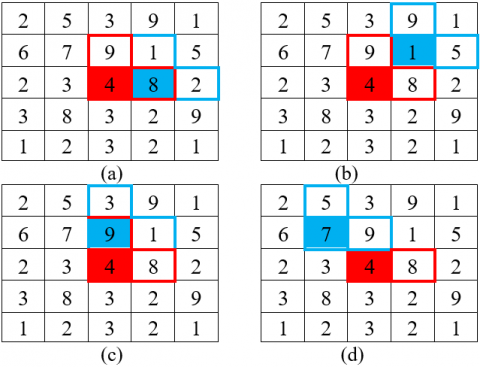
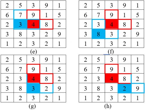
Figure 8. Calculation of tetra pattern bits for center pixel direction “1” using the direction of neighbours. Direction of center pixel (red) and neighborhood pixel (cyan)
Likely, the other tetra patterns for other directions of gc are converted to binary patterns. In total, it results in 12 patterns with 4 directions corresponding 3 patterns of each direction as shown in Figure 8.
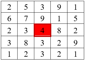
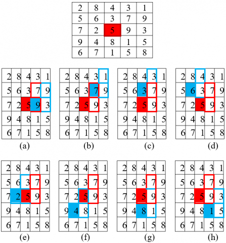
Below in Figure 9 shows example to obtain second order LTrP pattern and magnitude pattern on a patch of gray scale image.
Example:
Figure 9. For generating tetra pattern, bit is coded with 1 when the direction of the center pixel and its neighbor are different, otherwise "0". For Magnitude pattern, the bit is coded with "1" when the magnitude of center pixel is less than the magnitude of its neighbor, otherwise "0"
When we apply the first-order derivative for neighborhood pixel "8" in the horizontal and vertical direction we obtain direction "3" and magnitude "9.2". value "3" is assigned as the direction of center pixel and direction obtained from neighborhood pixel are not same. For magnitude pattern value "1" is assigned as the magnitude of center pixel is "6" which is less than the magnitude of neighborhood pixel. Likely, tetra pattern for center pixels having directions 2, 3, and 4 are computed.
Tetra pattern= 30340320
Pattern 1: 00000010
Pattern 2: 10100100
Pattern 3: 00010000
Magnitude pattern: 11100101
2.5 Local Vector Pattern (LVP)
The idea of LVP [10] is generating micro patterns of LVP by the vectors of each pixel that are constructed by calculating the values between the centre pixel and its neighborhood pixels with various distances of different directions by using an effective coding scheme called Comparative space transform (CST). Figure 10 shows pixel directions with refence to center pixel.
Figure 10. Adjacent pixels of Vβ,D(Gc) with directions
$\begin{array}{l}
\operatorname{LVP}_{\mathrm{P}, \mathrm{R}, \beta}\left(\mathrm{G}_{\mathrm{c}}\right) \\
=\left\{\mathrm{S}\left(\mathrm{V}_{\beta, \mathrm{D}}\left(\mathrm{G}_{1, \mathrm{R}}\right), \mathrm{V}_{\beta+45^{\circ}, \mathrm{D}}\left(\mathrm{G}_{1, \mathrm{R}}\right), \mathrm{V}_{\beta, \mathrm{D}}\left(\mathrm{G}_{\mathrm{c}}\right), \mathrm{V}_{\beta+45^{\circ}, \mathrm{D}}\left(\mathrm{G}_{\mathrm{c}}\right)\right),\right. \\
\qquad \begin{array}{c}
\mathrm{S}\left(\mathrm{V}_{\beta, \mathrm{D}}\left(\mathrm{G}_{2, \mathrm{R}}\right), \mathrm{V}_{\beta+45^{\circ}, \mathrm{D}}\left(\mathrm{G}_{2, \mathrm{R}}\right), \mathrm{V}_{\beta, \mathrm{D}}\left(\mathrm{G}_{\mathrm{c}}\right), \mathrm{V}_{\beta+45^{\circ}, \mathrm{D}}\left(\mathrm{G}_{\mathrm{c}}\right)\right), \\
\left.\ldots \ldots \mathrm{S}\left(\mathrm{V}_{\beta, \mathrm{D}}\left(\mathrm{G}_{\mathrm{p}, \mathrm{R}}\right), \mathrm{V}_{\beta+45^{\circ}, \mathrm{D}}\left(\mathrm{G}_{\mathrm{p}, \mathrm{R}}\right), \mathrm{V}_{\beta, \mathrm{D}}\left(\mathrm{G}_{\mathrm{c}}\right), \mathrm{V}_{\beta+45^{\circ}, \mathrm{D}}\left(\mathrm{G}_{\mathrm{c}}\right)\right)\right\} \\
\text { at } \mathrm{p}=1,2 \ldots 8
\end{array}
\end{array}$ (27)
S (...) adopts transform ratio which is calculated with a pair wise direction of vector of the reference pixel to transform the β-direction value of neighborhoods to (β+45°) direction, which is compared with the original (β+45°) direction value of neighborhoods for labeling the binary pattern of micro pattern.
S (.,.) can be defined as
$\begin{array}{l}
S\left(\mathrm{~V}_{\beta, \mathrm{D}}\left(\mathrm{G}_{\mathrm{p}, \mathrm{R}}\right), \mathrm{V}_{\beta+45^{\circ}, \mathrm{D}}\left(\mathrm{G}_{\mathrm{p}, \mathrm{R}}\right), \mathrm{V}_{\beta, \mathrm{D}}\left(\mathrm{G}_{\mathrm{c}}\right), \mathrm{V}_{\beta+45^{\circ}, \mathrm{D}}\left(\mathrm{G}_{\mathrm{c}}\right)\right) \\
=\left\{\begin{array}{l}
1, \text { if } \mathrm{V}_{\beta+45^{\circ}, \mathrm{D}}\left(G_{\mathrm{p}, \mathrm{R}}\right)-\left(\frac{\mathrm{V}_{\beta+45^{\circ}, \mathrm{D}}\left(\mathrm{G}_{\mathrm{c}}\right)}{\mathrm{V}_{\beta, \mathrm{D}}\left(\mathrm{G}_{\mathrm{c}}\right)} \mathrm{x} V_{\beta, \mathrm{D}}\left(\mathrm{G}_{\mathrm{p}, \mathrm{R}}\right)\right) \geq 0 \\
0, \text { else }
\end{array}\right.
\end{array}$ (28)
Finally, LVPP,R (Gc) at reference pixel Gc is concatenation of four 8-bit binary patterns LVPs.
$\mathrm{LVP}_{\mathrm{p}, \mathrm{R}}\left(\mathrm{G}_{\mathrm{c}}\right)=\left\{\mathrm{LVP}_{\mathrm{p}, \mathrm{R}, \beta}\left(\mathrm{G}_{\mathrm{c}}\right) \mid \beta=0^{\circ}, 45^{\circ}, 90^{\circ}, 135^{\circ}\right\}$ (29)
Example as shown in Figure 11 for encoding first order LVP pattern
Figure 11. Example of first order LVP in β=0° direction
By using the above equations
$\begin{array}{l}
\mathrm{LVP}_{\mathrm{P}, \mathrm{R}, 0^{\circ}}\left(\mathrm{G}_{\mathrm{c}}\right)=10000011 \\
\mathrm{LVP}_{\mathrm{p}, \mathrm{R}, 45^{\circ}}\left(\mathrm{G}_{\mathrm{c}}\right)=00111001 \\
\mathrm{LVP}_{\mathrm{p}, \mathrm{R}, 90^{\circ}}\left(\mathrm{G}_{\mathrm{c}}\right)=00101101 \\
\mathrm{LVP}_{\mathrm{p}, \mathrm{R}, 135^{\circ}}\left(\mathrm{G}_{\mathrm{c}}\right)=00101101
\end{array}$
Finally LVP is obtained by concatenating the four binary patterns in four directions
$\mathrm{LVP}_{\mathrm{p}, \mathrm{R}}\left(\mathrm{G}_{\mathrm{c}}\right)=10000011001110010010110100101101$
2.6 Local Anisotropic Pattern (LAP)
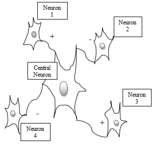
Difference of physical properties at different dimensions of an object is called anisotropy [11]. Applied for images it is taken as difference of statistical properties in different orientations. In primary visual cortex interaction between neurons, including excitation and inhibition are determined by correlation of their received stimuli. Cortical neurons with similar property have a higher probability of connection and interact by excitation, otherwise they interact by inhibition, called biological rule of synaptic plasticity. The interaction between two neurons can be estimated according to the degree of the similarity between their anisotropies. The interaction between neurons x and xi can be given as
$s\left(\mathrm{x}, \mathrm{x}_{\mathrm{i}}\right)=\left\{\begin{array}{l}
1 \text { if }|A(y)-A(y i)|<T \\
0 \text { otherwise }
\end{array}\right.$ (30)
Figure 12. Picture of Visual cortical neuron and its four adjacent neurons with different values of anisotropy ‘+’ denotes excitation, ‘-’ denotes inhibition
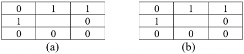
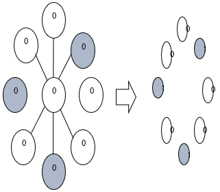
Figure 13. a), b) Picture of local anisotropic pattern. Adjacent neuron with similar anisotropy to the central neuron respond as excitation i.e., 1 and dissimilar ones respond as inhibition i.e. 0. The final pattern achieved as “00100101”
Figure 12 shows the picture of Visual cortical neuron and its adjacent neurons. In Image, anisotropy value of each pixel is calculated from grey level values and then to binary pattern. Binary patterns are converted into decimal number and accumulated as histogram which is used as feature vector as shown in Figure 13.
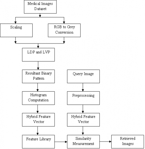
Many CBMIR systems are developed for image retrieval. The below Figure 14 shows two phases: one with storing features offline called as feature library and other with getting features of query image. The medical images are preprocessed with techniques [12] like scaling and RGB to grey conversion. Hybrid pattern [13] is formed by using local derivative pattern and local vector pattern of the preprocessed image. The features are compared with feature library using a similarity measurement.
Figure 14. CBMIR framework using Hybrid pattern
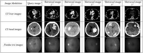
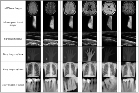
Figure 15 shows the result of retrieved images [14-16] using hybrid texture patterns with query using different medical images like CT liver, CT head, Fundus iris images, MRI brain images, Mammogram breast images, Ultrasound images, X-ray images of bone, X-ray images of chest, X-ray images of dental [17-19].
Figure 15. Image retrieval using hybrid pattern
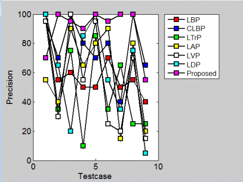
Performance analysis [20] of the system with hybrid features done by precision, recall and F1 score. Precision is defined as the ration of positive observations that are predicted exactly to the total number of observations that are positively retrieved.
$\text { Precision }=\frac{\text { True Positive }}{\text { True positive }+\text { False positive }}$ (31)
Recall is defined as the fraction of the relevant data that is successfully retrieved.
$\text { Recall }=\frac{\text { True Positive }}{\text { True positive }+\text { False negative }}$ (32)
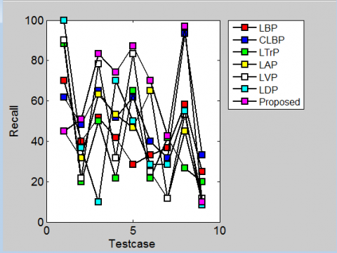
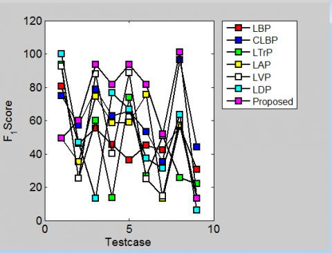
Figure 16, Figure 17 and Figure 18 shows precision, recall and f1 score respectively of the proposed system and compared with different patterns different sets.
Figure 16. Analysis of precision over different patterns to different datasets
Figure 17. Analysis of recall over different patterns to different datasets
Figure 18. Analysis of F1-scores over different patterns to different datasets
We proposed an efficient CBMIR model with hybrid pattern used based feature extraction using LVP and LDP. The proposed system gives satisfactory results to maximize recall, precision and f1 score when evaluated on publicly available different medical database. In future, we will focus on more different hybrid patterns using SIFT and SURF features.
|
LBP |
Local Binary Pattern |
|
CLBP |
Completed Local Binary Pattern |
|
LAP |
Local Anisotropic Pattern |
|
LDP |
Local Derivative Pattern |
|
LTrP |
Local Tetra Pattern |
|
LVP |
Local Vector Pattern |
[1] Rui, Y., Huang, T., Chang, S.F. (1997). Image retrieval: Past, present, and future. Proceedings of the International Symposium on Multimedia Information Processing, pp. 1-23.
[2] Huang, F., Jin, C., Zhang, Y., Weng, K., Zhang, T., Fan, W. (2018). Sketch-based image retrieval with deep visual semantic descriptor. Pattern Recognition, 76: 537-548. https://doi.org/10.1016/j.patcog.2017.11.032
[3] Müller, H., Michoux, N., Bandon, D., Geissbuhler, A. (2004). A review of content-based image retrieval systems in medical applications-clinical benefits and future directions. International Journal of Medical Informatics, 73(1): 1-23. https://doi.org/10.1016/j.ijmedinf.2003.11.024
[4] Shrivastava, N., Tyagi, V. (2014). Content based image retrieval based on relative locations of multiple regions of interest using selective regions matching. Information Sciences, 259: 212-224. https://doi.org/10.1016/j.ins.2013.08.043
[5] Lowe, D.G. (2004). Distinctive image features from scale-invariant keypoints. International Journal of Computer Vision, 60: 91-110. https://doi.org/10.1023/B:VISI.0000029664.99615.94
[6] Dubey, S.R., Singh, S.K., Singh, R.K. (2016). Local bit-plane decoded pattern: A novel feature descriptor for biomedical image retrieval. IEEE Journal of Biomedical and Health Informatics, 20(4): 1139-1147. https://doi.org/10.1109/JBHI.2015.2437396
[7] Zhang, B., Gao, Y., Zhao, S., Liu, J. (2010). Local derivative pattern versus local binary pattern: Face recognition with high-order local pattern descriptor. IEEE Transactions on Image Processing, 19(2): 533-544. https://doi.org/10.1109/TIP.2009.2035882
[8] Singh, S., Maurya, R., Mittal, A. (2012). Application of complete local binary pattern method for facial expression recognition. 2012 4th International Conference on Intelligent Human Computer Interaction (IHCI), Kharagpur, pp. 1-4. https://doi.org/10.1109/IHCI.2012.6481801
[9] Murala, S., Maheshwari, R.P., Balasubramanian, R. (2012). Local tetra patterns: A new feature descriptor for content-based image retrieval. IEEE Transactions on Image Processing, 21(5): 2874-2886. https://doi.org/10.1109/TIP.2012.2188809
[10] Hung, T., Fan, K. (2014). Local vector pattern in high-order derivative space for face recognition. 2014 IEEE International Conference on Image Processing (ICIP), Paris, pp. 239-243. https://doi.org/10.1109/ICIP.2014.7025047
[11] Du, S., Yan, Y., Ma, Y. (2017). LAP: a bio-inspired local image structure descriptor and its applications. Multimedia Tools and Applications, 76: 13973-13993. https://doi.org/10.1007/s11042-016-3779-2
[12] Cui, C., Lin, P., Nie, X., Yin, Y., Zhu, Q. (2017). Hybrid textual-visual relevance learning for content-based image retrieval. Journal of Visual Communication and Image Representation, 48: 367-374. https://doi.org/10.1016/j.jvcir.2017.03.011
[13] Cai, Y., Li, Y., Qiu, C., Ma, J., Gao, X. (2019). Medical image retrieval based on convolutional neural network and supervised hashing. IEEE Access, 7: 51877-51885. https://doi.org/10.1109/ACCESS.2019.2911630
[14] Shamna, P., Govindan, V.K., Abdul Nazeer, K.A. (2018). Content-based medical image retrieval by spatial matching of visual words. Journal of King Saud University - Computer and Information Sciences. https://doi.org/10.1016/j.jksuci.2018.10.002
[15] Mishra, S., Panda, M. (2018). Medical image retrieval using self-organising map on texture features. Future Computing and Informatics Journal, 3(2): 359-370. https://doi.org/10.1016/j.fcij.2018.10.006
[16] Ramos, J., Kockelkorn, T.T.J.P., Ramos, I., Ramos, R., Grutters, J., Viergever, M.A., van Ginneken, B., Campilho, A. (2016). Content-based image retrieval by metric learning from radiology reports: application to interstitial lung diseases. IEEE Journal of Biomedical and Health Informatics, 20(1): 281-292. https://doi.org/10.1109/JBHI.2014.2375491
[17] Shamna, P., Govindan, V.K., Abdul Nazeer, K.A. (2019). Content based medical image retrieval using topic and location model. Journal of Biomedical Informatics. https://doi.org/10.1016/j.jbi.2019.103112
[18] Tzelepi, M., Tefas, A. (2018). Deep convolutional learning for content based image retrieval. Neurocomputing, 275: 2467-2478. https://doi.org/10.1016/j.neucom.2017.11.022
[19] Ojala, T., Pietikainen, M., Maenpaa, T. (2000). Multiresolution gray scale and rotation invariant texture classification with local binary patterns. IEEE Transactions on Pattern Analysis and Machine Intelligence, 24(7): 971-987. https://doi.org/10.1109/TPAMI.2002.1017623
[20] Darapureddy, N., Karatapu, N., Battula, T.K. (2020). Optimal weighted hybrid pattern for content based medical image retrieval using modified spider monkey optimization. International Journal of Imaging Systems and Technology. https://doi.org/10.1002/ima.22475