Mohammad Takey Elias Kassim![]() | Emad Toma Karash*
| Emad Toma Karash*![]() | Jamal Nayief Sultan
| Jamal Nayief Sultan![]()
© 2023 IIETA. This article is published by IIETA and is licensed under the CC BY 4.0 license (http://creativecommons.org/licenses/by/4.0/).
OPEN ACCESS
The beams are frequently utilized in construction as well as in the fabrication of vehicles like as trains, ships, and airplanes. Depending on the necessary working circumstances, several materials may have been utilized in the production of these beams, from high fatigue resistance, high corrosion resistance, strong earthquake resistance, and other aspects. As a result, composite beams made of glass or carbon fibers are increasingly commonly employed. This is a result of its strong collapse resistance, light weight, and strong fatigue stress resistance. In order to compare the models' resistance to deformations, stresses, and strains that they are exposed to during loading, this article focuses on constructing a variety of models using a variety of composite materials and shapes. The outcomes demonstrate a rise in the rate of deformation. against beams with linear shapes in those with non-linear shapes. Additionally, the findings demonstrate an increase in stresses and strains in regions with curves (i.e., areas that are nonlinear).
fiberglass, carbon fiber, steel, concrete, beams, Finite element method
Partial or total contact between the two elements occurs when two elements that can withstand bending moments are elastically coupled at the interface. If the elastic connection is flexible, there will be differential axial strains at the common interface that cause slip, and there may also be differential deflections that cause uplift between the two parts. The majority of composite structures are dimensionally reducible, and utilizing lower-dimensional structural models, their analysis can be accelerated [1]. This article develops a composite beam element that can be used to simulate the nonlinear behavior of composite beams. It was discovered that at the same load level, increasing the cover plate's thickness increased the final load while decreasing the maximum slide [2]. One-dimensional beam models, for instance, can depict thin structural elements where the length is substantially more than the cross-sectional dimension. Although beam theory has been available for many centuries, it wasn't until about 1985 that academics started to concentrate largely on developing beam models for structures with arbitrary cross-sections and composite materials [3]. The efficient high-fidelity approach developed by Hodges and his coworkers stands out significantly in the quest for effective yet accurate models appropriate for nonlinear analysis of composite beams and is gaining acceptance in both industry and the scientific community [4]. Both in elastic and inelastic areas, fiber-reinforced plastic composites (FRP) have physically nonlinear features. If lamina shear stressors reach a 5 reasonably substantial ratio to longitudinal tensile stresses, they are known to be the main cause of elastic nonlinearity. In this case, the mechanical performance of the composites is dominated by the resin matrix. The in-plane shear responses of FRP plies are nonlinear over the whole range investigated because the shear stress-strain responses of polymer resins are nonlinear over the entire strain range and at extremely low strain levels [5, 6]. Able to predict failure brought on by stress concentrations with accuracy [7, 8]. The Ramberg-Osgood equation [9], which is also common in investigations of metal fatigue, is another widely used model. The use of mathematical curve fitting functions provides a more adaptable description methodology [10-12]. Results from Matrix 3D are contrasted with those from the reputable commercial structural analysis program SAP2000. When compared to SAP2000, Matrix 3D's non-linear analysis solver performed better when computing a given structure with hinges that were modelled at element ends [13]. The usage of sophisticated and complicated finite element structural analysis computer programs has been made possible by the consistent advancement of computer technology over the past ten years. Commercial and non-commercial structural analysis programs generally fall into two categories [14-17]. It is important to take convergence issues into account when using finite element programs for sophisticated non-linear calculations. When non-linear constitutive relations, in particular softening ones, are added to FE non-linear investigations, the software solver encounters convergence issues in addition to explicit numerical approaches. In order to obtain any findings from the problematic FE system, users typically turn to explicit dynamic analysis [18, 19]. Contrary to non-linear static and implicit dynamic analyses, which are iterative, explicit dynamic analyses do not converge to solution in iterations. Therefore, in order to examine the outcomes of explicit dynamic analysis, extra steps are necessary. In this regard, it is advantageous for the field of non-linear structural analysis to investigate whether computation convergence may be enhanced using non-linear static or implicit dynamic approaches [20, 21]. The publications by Najem et al. [22], Avalon and Donaldson [23], Vershchaka et al. [24], Ranz et al. [25], Vereshaka and Karash [26] appear to be the only ones for the case of thin-walled curved beams made of isotropic materials that fully take into account shear deformability. Palanim and Rajasekaran [27] has created a stability study for laminated, curved thin-walled beams without taking shear effects into account. In any case, relatively few studies have taken into account the flexibility caused by warping shear in addition to flexural shear when studying the mechanics of curved thin-walled beams made of composite materials. In order to assess the mechanics of out-of-plane movement. [28, 29] developed a model that takes into account the full shear flexibility in curved beams made of laminated composite materials. The paradigm given by Cortínez et al. [28] and Liu et al. [29] is only truly applicable in balanced symmetrical or particularly orthotropic situations. In a variety of industries, including aeronautics, the marine sector, energy, and civil construction, composite materials with geometry that incorporates significant bending radii are frequently used in engineering constructions [30]. Interlayer delamination results from the breakdown of these components, which is mostly caused by interlinear tensile strength [31] In order to obtain an effective design, it is essential to determine interlinear tensile strength (ILTS). To determine ILTS, a variety of experimental techniques are available.
In this article, nine mathematical models of beams will be designed and made up of different composite materials and in different shapes (straight, twisted, arched), in order to compare between deformations, stresses and strains when a high load is placed on them using the ANSYS-15.0 program, and this study differs from previous studies because it takes Linear and other non-linear models have the same dimensions, and the results are compared for all models. The last paragraphs of the article are as follows: The material used and the mathematical model, Results and Discussion, Conclusions, Acknowledgment, future studies and references.
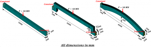
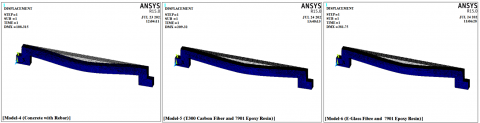
The ANSYS-15 program was used to create nine 3D models of three different types of beams. Three models are made of traditional materials (Concrete and Rebar), and the three models are made of composite materials (T300 Carbon Fiber and 7901 Epoxy Resin), and three models are composed of composite materials (E-Glass Fibre and 7901 Epoxy Resin), and exerting a force load (10 MN) in the direction of the vertical axis (y) into the center of the top surface of each of the nine models.
Figure 1. It shows the shapes of the models used in the tests and the points of loading them
Table 1. Describe the mechanical properties of fiberglass, jute, carbon fiber, and concrete composition [18, 29-33]
|
Model |
Materials |
Density,ρ, (Kg/M-3) |
Modulus of Elasticity, E, (GPa) |
Passion's Ratio |
Modulus of Rigidity, G, (GPa) |
Number of Layers |
Price Kilograms, \$ |
|
|
M-1 |
Concrete and Rebar |
Concrete, 93% |
2400 |
27 |
0.21 |
21 |
10 |
0.125 |
|
Rebar, 7% |
7850 |
200 |
0.3 |
78 |
0.65 |
|||
|
M-2 |
T300 Carbon Fiber and 7901 Epoxy Resin |
T300 carbon fiber, 55% |
1760 |
240 |
0.25 |
40 |
20 |
14 |
|
7901 Epoxy Resin, 45% |
1150 |
3.2 |
0.35 |
1.19 |
0.05 |
|||
|
M-3 |
E-Glass Fibre and 7901 Epoxy Resin |
E-Glass Fibre, 55% |
2580 |
72.3 |
0.2 |
30 |
20 |
0.715 |
|
7901 Epoxy Resin, 45% |
1150 |
3.2 |
0.35 |
1.19 |
0.05 |
|||
|
M-4 |
Concrete and Rebar |
Concrete, 93% |
2400 |
27 |
0.21 |
21 |
10 |
0.125 |
|
Rebar, 7% |
7850 |
200 |
0.3 |
78 |
|
0.65 |
||
|
M-5 |
T300 Carbon Fiber and 7901 Epoxy Resin |
T300 carbon fiber, 55% |
1760 |
240 |
0.25 |
40 |
20 |
14 |
|
7901 Epoxy Resin, 45% |
1150 |
3.2 |
0.35 |
1.19 |
|
0.05 |
||
|
M-6 |
E-Glass Fibre and 7901 Epoxy Resin |
E-Glass Fibre, 55% |
2580 |
72.3 |
0.2 |
30 |
20 |
0.715 |
|
7901 Epoxy Resin, 45% |
1150 |
3.2 |
0.35 |
1.19 |
|
0.05 |
||
|
M-7 |
Concrete and Rebar |
Concrete, 93% |
2400 |
27 |
0.21 |
21 |
10 |
0.125 |
|
Rebar, 7% |
7850 |
200 |
0.3 |
78 |
|
0.65 |
||
|
M-8 |
T300 Carbon Fiber and 7901 Epoxy Resin |
T300 carbon fiber, 55% |
1760 |
240 |
0.25 |
40 |
20 |
14 |
|
7901 Epoxy Resin, 45% |
1150 |
3.2 |
0.35 |
1.19 |
|
0.05 |
||
|
M-9 |
E-Glass Fibre and 7901 Epoxy Resin |
E-Glass Fibre, 55% |
2580 |
72.3 |
0.2 |
30 |
20 |
0.715 |
|
7901 Epoxy Resin, 45% |
1150 |
3.2 |
0.35 |
1.19 |
|
0.05 |
||
Figure 2. It shows the paths that were taken on the different models
Table 2. The results of the mechanical characteristics of the composite materials obtained by using a Mathcad -15 program
|
Models |
Materials and the ratios of the materials |
Code [0] |
Code [90] |
||||
|
Eii, MPa |
Gij, MPa |
μij |
Eii, MPa |
Gij, MPa |
μij |
||
|
M-1 M-4 M-7 |
Concrete and Rebar |
E11=205650 E22=100000 E33=111100 |
G12=70400 G13=76420 G23=49310 |
μ12=0.294 μ13=0.214 μ23=0.217 |
E11=108000 E22=205600 E33=110500 |
G12=70400 G13=49310 G23=76420 |
μ12=0.294 μ13=0.217 μ23=0.214 |
|
M-2 M-5 M-8 |
T300 Carbon Fiber and 7901 Epoxy Resin |
E11=143300 E22=12420 E33=18680 |
G12=3983 G13=4331 G23=2794 |
μ12=0.271 μ13=0.347 μ23=0.347 |
E11=12420 E22=143300 E33=18680 |
G12=3983 G13=2794 G23=4331 |
μ12=0.2 μ13=0.347 μ23=0.347 |
|
M-3 M-6 M-9 |
E-Glass Fibre and 7901 Epoxy Resin |
E11=51090 E22=12130 E33=13790 |
G12=3989 G13=4331 G23=2794 |
μ12=0.061 μ13=0.346 μ23=0.346 |
E11=12130 E22=51090 E33=13790 |
G12=3989 G13=2794 G23=4331 |
μ12=0.061 μ13=0.346 μ23=0.346 |
Table 3. The materials, codes, models, forms, load types, and element types that are utilized in the ANSYS 15.0 application
|
No. |
Material |
Code |
Model |
Individual disciplines |
Type of ELEMENT |
|
1 |
Model - 1 |
[0/90/0/90/0/90/0/90/0/90] |
Linear, (Orthotropic) |
Structural |
SHELL 281 |
|
2 |
Model - 2 |
[0/90/0/90/0/90/0/90/0/90/0/ 90/0/90/0/90/0/90/0/90] |
Linear, (Orthotropic) |
||
|
3 |
Model - 3 |
[0/90/0/90/0/90/0/90/0/90/0/ 90/0/90/0/90/0/90/0/90] |
Linear, (Orthotropic) |
||
|
4 |
Model - 4 |
[0/90/0/90/0/90/0/90/0/90] |
Non-Linear |
||
|
5 |
Model - 5 |
[0/90/0/90/0/90/0/90/0/90/0/ 90/0/90/0/90/0/90/0/90] |
Non-Linear |
||
|
6 |
Model - 6 |
[0/90/0/90/0/90/0/90/0/90/0/ 90/0/90/0/90/0/90/0/90] |
Non-Linear |
||
|
7 |
Model - 7 |
[0/90/0/90/0/90/0/90/0/90] |
Non-Linear |
||
|
8 |
Model - 8 |
[0/90/0/90/0/90/0/90/0/90/0/ 90/0/90/0/90/0/90/0/90] |
Non-Linear |
||
|
9 |
Model - 9 |
[0/90/0/90/0/90/0/90/0/90/0/ 90/0/90/0/90/0/90/0/90] |
Non-Linear |
Figure 1 depicts the simulation model's geometry as well as the model's direction of load application. Figure 2 depicts the routes taken on the nine models to determine the deformations, stresses, and strains that these models experience when a load is applied to the center of their upper surfaces and its value is (10 MN). The mechanical and other details of the nine models are displayed in Table 1. Additionally, it displays the components and ratios created, including any models created using the ANSYS -15.0 program. The mechanical properties of various compound materials are shown in Table 2 and were calculated using the Mathcad - 15 application. Several models were employed to get the best values for the materials' respective moduli of elasticity, rigidity, and passions ratio. The materials, codes, models, load types, and element types used in the ANSYS-15.0 program are listed in Table 3.
Nine mathematical models were created for three distinct forms and three different composite material mixtures, and they were tested in the ANSYS 15.0 program with a load of (10 MN) applied to the upper surface of each model while the sides of the models remained fixed while the load was shed, to determine the deformations, stresses, and strains that these models are subjected to when the load is applied, and the following findings were made:
3.1 Models (M-1, M-2, M-3)
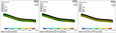
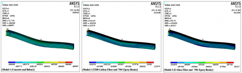
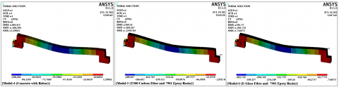
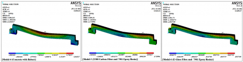
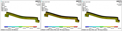
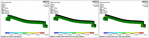
The three models (1, 2, and 3), which are composed of various composite materials but have the same geometric design, were tested, and the findings are shown in the Figures 3-15. The results of the deflection (δ) for these models are shown in Figure 3, and the results show that the deflection values for the three models are, as is abundantly obvious (δ1=72.77 mm, δ2=153.11 mm, and δ3= 351.79 mm). The results of the component of the displacement in a direction (x), for these models are shown in Figure 4, The displacement outcomes are shown in the figure as follows, (Ux1=- 26.24 to 26.24 mm, Ux2=- 8.39 to 8.41 mm, and Ux3=- 25.97 to 29.99 mm). Figure 5 shows the models' results for the component of displacement in a direction (y), the figure suggests that the results' values are, (Uy1=72.77 mm, Uy2=153.11 mm, and Uy3= 351.79 mm). Figure 6 shows the components of these models' displacements in a direction (z), according to the figure, displacement values might be either positive or negative are (Uz1=- 0.0046 to 0.0327 mm, Uz2=- 0.0187 to 0.1923 mm, and Uz3=- 0.0058 to 0.0496 mm). The results of the normal stress (σx) for these models are shown in Figure 7. The outcomes of this stresses show the values (σx1=- 4029.13 to 2739.6 MPa, σx2=- 9029.29 to 4261.27 MPa, and σx3=- 3913.65 to 2517.31 MPa). The results of the typical stress (σy), as shown Figure 8, the figure displays the effects of this stress for several models, with values ranging from $\begin{aligned} & \left(\sigma_{y_1}=-2906.21 \text { to } 756.97 \mathrm{MPa}, \sigma_{y_2}=\right. \left.-3633.4 \text { to } 1103.9 \mathrm{MPa} \text {, and } \sigma_{y_3}=-2616.15 \text { to } 917.49 \mathrm{MPa}\right) \text {. }\end{aligned}$ Figure 9 displays the shear stress (τxy) findings for these models, the figure demonstrates that the shear stresses values range from $\begin{aligned} & \quad\left(\tau_{x y_1}=-1928.51 \text { to } 1929.26 \mathrm{MPa}, \tau_{x y_2}=\right.-1695.37 \text { to } 1696.03 \mathrm{MPa} \text {, and } \tau_{x y_3}= -1750.01 \text { to } 1750.51 \mathrm{MPa}) .\end{aligned}$ The greatest stress intensity (σint.) values for the three models are shown in figure 10 results of the stresses intensity (σint.), and they were $\begin{aligned} & \left(\sigma_{\text {int.}_1}=5466.95 \mathrm{MPa}, \sigma_{\text {int.}_2}=9518.33 \mathrm{MPa} \text {, and } \sigma_{\text {int. }_3}=\right. 5130.09 \mathrm{MPa}) .\end{aligned}$ The results of the normal strain (εx), for three models, are shown in Figure 11, and the figure demonstrates that this strain's value fall within the following range $\begin{gathered}\left(\varepsilon_{x_1}=-0.0117 \text { to } 0.0113, \varepsilon_{x_2}=-0.0285 \text { to } 0.0168 \text { and } \varepsilon_{x_3}\right. =-0.0635 \text { to } 0.0485) .\end{gathered}$ Figure 12 shows the outcomes of these models' normal strains (εy), and the figure shows that the values of this strain range between the following values $\begin{aligned} \left(\varepsilon_{y_1}=-0.0161 \text { to } 0.0105, \varepsilon_{y_2}=\right. \left.-0.1328 \text { to } 0.0962 \text {, and } \varepsilon_{y_3}=-0.1961 \text { to } 0.0785\right)\end{aligned}$. The results of the normal strain (εz), for three models, are shown in Figure 13, the values of the results show that the strains have values between $\begin{aligned} & \quad\left(\varepsilon_{z_1}=-0.0043 \text { to } 0.0099, \varepsilon_{z_2}=\right. \left.-0.0345 \text { to } 0.1233 \text {, and } \varepsilon_{z_3}=-0.0210 \text { to } 0.1011\right) .\end{aligned}$ Figure 14 displays the results of the shear strain (εxy) for three models, this strain's value, according to the figure, fall within the following range $\begin{aligned} & \left(\varepsilon_{x y_1}=-0.0273 \text { to } 0.0274, \varepsilon_{x y_2}=\right. \left.-0.4256 \text { to } 0.4258 \text {, and } \varepsilon_{x y_3}=-0.4357 \text { to } 0.4388\right)\end{aligned}$. Figure 15 displays the findings of the models (1, 2, and 3) for the intensity strain (εxy); the figure reveals that the three models' maximum strain values were $\left(\varepsilon_{\text {int. } 1}=0.0376, \varepsilon_{i n t .2}=0.4424\right.$, and $\left.\varepsilon_{\text {int }_{\cdot 3}}=0.4599\right)$.
Figure 3. Results of the deflection (δ), for models (1, 2, and 3)
Figure 4. Results of the component of the displacement in a direction (Ux), for models (1, 2, and 3)
Figure 5. Results of the component of the displacement in a direction (Uy), for models (1, 2, and 3)
Figure 6. Results of the component of the displacement in a direction (Uz), for models (1, 2, and 3)
Figure 7. Results of the normal stress (σx), for models (1, 2, and 3)
Figure 8. Results of the normal stress (σy), for models (1, 2, and 3)
Figure 9. Results of the shear stress (τxy), for models (1, 2, and 3)
Figure 10. Results of the intensity stress (σint.), for models (1, 2, and 3)
Figure 11. Results of the normal strain (εx), for models (1, 2, and 3)
Figure 12. Results of the normal strain (εy), for models (1, 2, and 3)
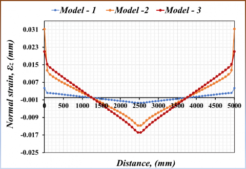
Figure 13. Results of the normal strain (εz), for models (1, 2, and 3)
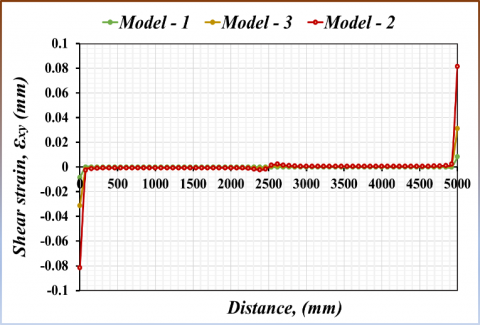
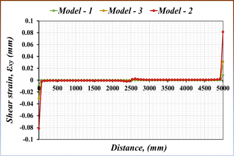
Figure 14. Results of the shear strain (εxy), for models (1, 2, and 3)
Figure 15. Results of the intensity strain (εint.)), for models (1, 2, and 3)
Figure 16. Compares the results of the relationship between displacement (Ux) and distance on a linear path (A-A), for models (1, 2, and 3)
Figure 17. Compares the results of the relationship between displacement (Uy) and distance on a linear path (A-A), for models (1, 2, and 3)
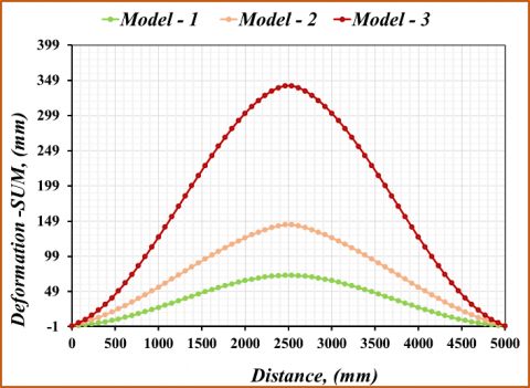
Figure 18. Compares the results of the relationship between displacement (Usum) and distance on a nonlinear path (A-A), for models (1, 2, and 3)
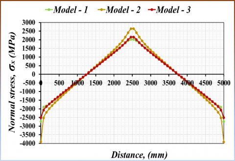
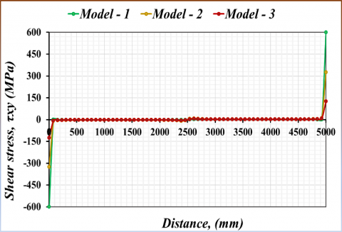
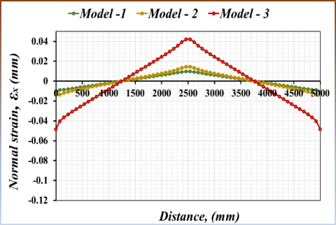
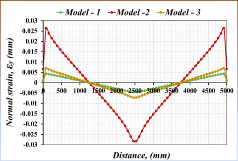
The results in the Figures 16-27 compare the deformations, stresses, and strains that the beams are subjected to when they are fixed to the sidewalls and a load is applied to them in the middle of the surface of the models using ANSYS – 15.0 program. From the start of the models to their end, as indicated by the path (A - A) in the Figure 2. The findings indicate that: Figure 16 compares the findings of different models for the relationship between displacement (Ux) and distance on a linear path (A-A). The results of various models for the relationship between displacement (Ux) and distance on a linear path (A-A) are compared in Figure 16, the findings show that the highest displacement values were in the model (M-3), where the highest displacement negative value (25.968 mm) was at distance (1230.8 mm) and the highest displacement positive value (25.941 mm) was at distance (3692.3 mm). Figure 17 compares the findings for various models' linear route (A-A) relationship between displacement (Uy) and distance, the figure demonstrates that the model (M-3) experienced the greatest displacement, with the greatest downward displacement of (341.04 mm) occurring at the distance (2540 mm). The relationship between displacement (Usum) and distance on a linear path (A-A), for three models, is compared in Figure 18, According to the data shown in the figure, the distance (2538.5 mm) recorded the highest values of displacement (Usum), and its value was (341.04 mm) for the model (M-3). Figure 19 compares the findings for three models for the relationship between normal stress (σx) and distance on a linear path (A-A), and the figure shows that the highest normal stress values were recorded for the model (M-2), and the stress value (2629.5 MPa) was at the distance (2500 mm). Figure 20 compares the outcomes for different models for the relationship between normal stress (σy) and distance on a linear path (A-A), The highest normal stress (σy) was for the model (M-2), and its highest value was measured at the distance (2500 mm), The figure indicated that, and its value was (226.74 MPA). Figure 21 illustrates the comparison of the outcomes for different models for the relationship between shear stress (τxy) and distance along a linear path (A-A), and the figure depicts the maximum shear stress value (τxy) recorded for the model (M-1), where the value of this negative shear stress (600 MPa) was at the distance (0 mm), while the highest positive shear stress values were at the distance (5,000 mm), where its value was (600 MPa). According to the statistics in Figure 22, the second model had the highest stress intensity value (σint.), which compares the results of the relationship between distance on a linear path (A-A) and stress intensity (σint.) for three models, with the first value (3950 MPa) at the distance of (0 mm), the second value (2,630 MPa) at the distance of (2,500 mm), and the third value at the distance of (5,000 mm) and its value (3,950 MPa). Figure 23 compares the outcomes of the relationship between normal strain (εx) and distance on a linear path (A-A), for three models, and the figure demonstrates that the model (M-3) had values of the largest strain, with the highest negative strain value being recorded at distances of (0 and 5,000 mm), and its value being (0.04859), while the greatest positive strain measurements were (0.0419) and at a distance (2,500 mm). Figure 24 Compare the results of the relationship between normal strain (εy) and distance on a linear path (A-A), for these models, and the figure demonstrates that the model (M-3) recorded the largest strain value, and the stress value was (0.0283) at the distance (2,500 mm). Figure 25 compares the findings for three models' normal strain (εz) and distance on a linear path (A-A) relationships, and the findings of this strain in this figure demonstrate that the second model had the maximum negative strain, with a value of (0.0312) at the two distances (0, 5,000 mm), but the third model had the maximum negative strain, and its value (0.0158 mm) when viewed from a distance (2,500 mm). Figure 26 Compare the results of the relationship between shear strain (εxy) and distance on a linear path (A-A), for these three models, and the data in the figure, the third model had the maximum shear strain (εxy) and that its maximum negative shear strain value was (0.0815) at a distance (0 mm), in contrast, the greatest positive shear strain measurement (0.0815) was at a distance (5,000 mm). Figure 27 compares the outcomes of the relationship between distance on a linear path (A-A) and intensity strain (εint.), for the models (M-1, M-2, M-3), and the figure demonstrates that the second model had the maximum strain intensity values, with its value (0.0839) at a distance (0 mm).
Figure 19. Compares the results of the relationship between normal stress (σx) and distance on a linear path (A-A), for models (1, 2, and 3)
Figure 20. Compares the results of the relationship between normal stress (σy) and distance on a linear path (A-A), for models (1, 2, and 3)
Figure 21. Compares the results of the relationship between shear stress (τxy) and distance on a nonlinear path (A-A), for models (1, 2, and 3)
Figure 22. Compares the results of the relationship between stress intensity (σintesity) and distance on a linear path (A-A), for models (1, 2, and 3)
Figure 23. Compares the results of the relationship between normal strain (εx) and distance on a linear path (A-A), for models (1, 2, and 3)
Figure 24. Compare the results of the relationship between normal strain (εy) and distance on a linear path (A-A), for models (1, 2, and 3)
Figure 25. Compare the results of the relationship between normal strain (εz) and distance on a linear path (A-A), for models (1, 2, and 3)
Figure 26. Compare the results of the relationship between shear strain (εxy) and distance on a linear path (A-A), for models (1, 2, and 3)
Figure 27. Compare the results of the relationship between intensity strain (εint.) and distance on a linear path (A-A), for models (1, 2, and 3)
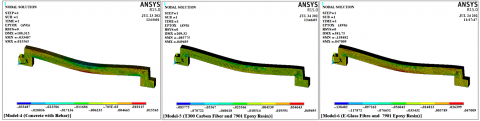
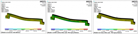
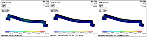
3.2 Models (M-4, M-5, M-6)
The ANSYS 15.0 program was used to test the three models (4, 5, and 6), which are made of different composite materials but have the same geometric design. The results are displayed in the Figures 28-40. The results of the deflection (δ) for these models are shown in Figure 28, and the results show that the deflection values for the three models are, as is abundantly obvious $\left(\delta_4=108.315 \mathrm{~mm}, \delta_5=209.32 \mathrm{~mm}\right.$, and $\left.\delta_6=381.75 \mathrm{~mm}\right)$. The results of the component of the displacement in a direction (x), for these models are shown in Figure 29, The displacement outcomes are shown in the figure as follows, $\begin{aligned} & \quad\left(\mathrm{Ux}_4=-12.291 \text { to } 12.634 \mathrm{~mm}, \mathrm{Ux}_5=\right. \left.-22.277 \text { to } 15.045 \mathrm{~mm}, \text { and } \mathrm{Ux}_6=-42.614 \text { to } 34.993 \mathrm{~mm}\right) .\end{aligned}$ Figure 30 shows the models' results for the component of displacement in a direction (y), the figure shows that the maximum results' values are, $\left(\mathrm{Uy}_4=108.296 \mathrm{~mm}, \mathrm{Uy}_5=209.267 \mathrm{~mm}, \text { and } \mathrm{Uy}_6=\right. 381.732 \mathrm{~mm})$. Figure 31 shows the components of these models' displacements in a direction (z), according to the figure, displacement values might be either positive or negative ar $\begin{aligned} & \left(\mathrm{Uz}_4=-0.3022 \text { to } 2.043 \mathrm{~mm}, \mathrm{Uz}_5=\right. \left.-0.1634 \text { to } 0.1729 \mathrm{~mm} \text {, and } \mathrm{Uz}_6=-0.0363 \text { to } 0.0537 \mathrm{~mm}\right) \text {. }\end{aligned}$ The results of the normal stress (σx) for these models are shown in Figure 32, the outcomes of this stresses show the values $\begin{aligned} & \quad\left(\sigma_{x_4}=-4450.28 \text { to } 1771.53 \mathrm{MPa}, \sigma_{x_5}=\right. -8693.53 \text { to } 3401.96 \mathrm{MPa} \text {, and } \sigma_{x_6}= -3927.74 \text { to } 2160.15 \mathrm{MPa}) .\end{aligned}$ The results of the typical stress (σy), as shown Figure 33, the figure displays the effects of this stress for several models, with values ranging from $\begin{aligned} & \left(\sigma_{y_4}=-3663.68 \text { to } 1588.22 \mathrm{MPa}, \sigma_{y_5}=\right. -5930.38 \text { to } 1722.76 \mathrm{MPa}, \text { and } \sigma_{y_6}= -3025.11 \text { to } 1072.91 \mathrm{MPa}) .\end{aligned}$ The results of the shear stress (τxy), for these models, are shown in Figure 34, the figure demonstrates that the shear stresses values range from ($\tau_{x y_1}=-1928.51$ to $1929.26 \mathrm{MPa}$, $\tau_{x y_2}=-1695.37$ to $1696.03 \mathrm{MPa}$ and $\tau_{x y_3}=-1750.01$ to $1750.5$) The greatest stress intensity (σint.) values for the three models are shown in Figure 35 results of the stresses intensity (σint.), and they were $\left(\sigma_{\text {int. }{ }_4}=7369.18 \mathrm{MPa}, \sigma_{\text {int. } 5}=9057.31 \mathrm{MPa}\right.$, and $\sigma_6=$ 4869.94 MPa). The results of the normal strain (εx), for three models, are shown in Figure 36, and the figure demonstrates that this strain's value fall within the following range $\begin{aligned} & \left(\varepsilon_{x_4}=-0.0334 \text { to } 0.0155, \varepsilon_5=\right. \left.-0.0857 \text { to } 0.0496, \text { and } \varepsilon_{x_6}=-0.1384 \text { to } 0.0470\right) .\end{aligned}$ Figure 37 shows the outcomes of these models' normal strains (εy), and the figure shows that the values of this strain range between the following values $\begin{aligned} \left(\varepsilon_{y_4}-0.0239 \text { to } 0.0109, \varepsilon_{y_5}=\right. \left.-0.0584 \text { to } 0.0496 \text {, and } \varepsilon_{y_6}=-0.2055 \text { to } 0.0805\right).\end{aligned}$ The results of the normal strain (εz), for three models, are shown in Figure 38, the values of the results show that the strains have values between $\begin{aligned} & \quad\left(\varepsilon_4=-0.0039 \text { to } 0.0123, \varepsilon_{z_5}=\right. \left.-0.0201 \text { to } 0.1163 \text {, and } \varepsilon_{z_6}=-0.0164 \text { to } 0.0958\right) \text {. }\end{aligned}$ Figure 39 displays the results of the shear strain (εxy) for three models, this strain's value, according to the figure, fall with in the following range $\begin{aligned} & \left(\varepsilon_{x y_4}=-0.0473 \text { to } 0.0505, \varepsilon_{x y_5}=\right. \left.-0.4439 \text { to } 0.3196, \text { and } \varepsilon_{x y_6}=-0.4443 \text { to } 0.3435\right).\end{aligned}$ The results of the models (4, 5, and 6) for the intensity strain (εxy) are shown in Figure 40, and the figure reveals that the three models' maximum strain values were $\left(\varepsilon_{\text {int }{ }_{.4}}=0.0581, \varepsilon_{\text {int. } .5}=0.4471\right.$, and $\left.\varepsilon_{\text {int. } 6}=0.4473\right)$.
Figure 28. Results of the deflection (δ), for models (4, 5, and 6)
Figure 29. Results of the displacement component in a direction (x), for models (4, 5, and 6)
Figure 30. Results of the displacement component in a direction (y), for models (4, 5, and 6)
Figure 31. Results of the displacement component in a direction (z), for models (4, 5, and 6)
Figure 32. Results of the normal stress (σx), for models (4, 5, and 6)
Figure 33. Results of the normal stress (σy), for models (4, 5, and 6)
Figure 34. Results of the shear stress (τxy), for models (4, 5, and 6)
Figure 35. Results of the intensity stress (σint.), for models (4, 5, and 6)
Figure 36. Results of the normal strain (εx), for models (4, 5, and 6)
Figure 37. Results of the normal strain (εy), for models (4, 5, and 6)
Figure 38. Results of the normal strain (εz), for models (4, 5, and 6)
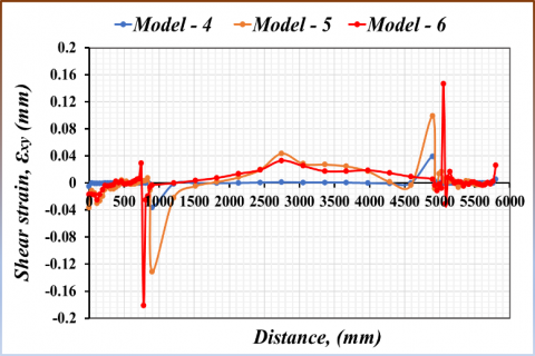
Figure 39. Results of the shear strain (εxy), for models (4, 5, and 6)
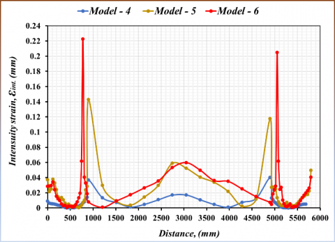
Figure 40. Results of the intensity strain (εint.), for models (4, 5, and 6)
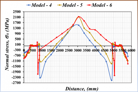
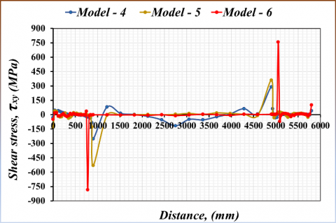
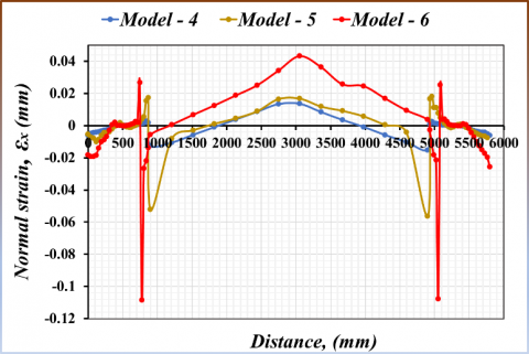
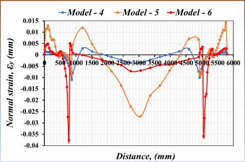
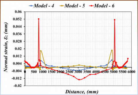
The ANSYS-15.0 program's results are shown in the Figures 41-52 and compare the deformations, stresses, and strains that the beams experience when they are fastened to the sidewalls and a load is applied to them in the center of the surface of the models. The path (B - B) in the figure represents the path from the beginning of the models to their end (2). The results show that: The results of various models for the relationship between displacement (Ux) and distance on a nonlinear path (B - B) are compared in Figure 41, the findings show that the highest displacement values were in the model (M-5), where the highest displacement negative value (14.146 mm) was at distance (1820 mm) and the highest displacement positive value (8.581 mm) was at distance (4280 mm). Figure 42 compares the findings for various models' nonlinear route (B - B) relationship between displacement (Uy) and distance, the figure demonstrates that the model (M-6) experienced the greatest displacement, with the greatest downward displacement of (371.77 mm) occurring at the distance (3050 mm). The relationship between displacement (Usum) and distance on a nonlinear path (B - B), for three models, is compared in Figure 43, According to the data shown in the figure, the distance (3053.8 mm) recorded the highest values of displacement (Usum), and its value was (371.8 mm) for the model (M-6). Figure 44 compares the findings for three models for the relationship between normal stress (σx) and distance on a nonlinear path (B - B), and the figure shows that the highest normal stress values were recorded for the model (M-4), and the stress value (2130.8 MPa) was at the distance (3053.8 mm). Figure 45 compares the outcomes for different models for the relationship between normal stress (σy) and distance on a nonlinear path (B - B), The highest normal stress (σy) was for the model (M-4), and its highest value was measured at the distance (4900 mm), according to the figure, and its value was (2284.9 MPa). Figure 46 illustrates the comparison of the outcomes for different models for the relationship between shear stress (τxy) and distance along a nonlinear path (B - B), and the figure depicts the maximum shear stress value (τxy) recorded for the model (M-6), where the value of this negative shear stress (783.66 MPa) was at the distance (776.92 mm), while the highest positive shear stress values were at the distance (5053.8 mm), where its value was (759.52 MPa). Figure 47 compares the outcomes of the relationship between distance on a nonlinear path (B - B) and stress intensity (σint.) for three models, and the data in the figure clearly show that the second model had the highest value of stress intensity (σint.), with the first value (2789.9 MPa) at the distance of (776.92 mm), the second value (2755.2 MPa) at the distance of (5053.8 mm). The results of the relationship between normal strain (εx) and distance on a nonlinear path (B - B) for three models are compared in Figure 48. The figure shows that the model (M-6) had values of the largest strain, with the highest negative strain value being recorded at distances of (776.62 and 5053.8 mm) and its value being (0.01085), while the greatest positive strain measurements were (0.0432 mm) and at a distance of (5053.8 mm) (3053.8 mm). Figure 49 Compare the results of the relationship between normal strain (εy) and distance on a nonlinear path (B - B), for these models, and the figure demonstrates that the model (M-6) recorded the largest strain value, and the stress value was (0.0375) at the distance (776.92 mm). Figure 50 compares the results for the relationships between normal strain (εz) and distance on a nonlinear path (B - B) for three models. The results show that the model (M-6) had the maximum negative strain, with a value of (0.0522) at the two distances (776.92, 3,053.8 mm), but the model (M-6) had the maximum negative strain, and its value (0.0134) when viewed from a distance (3053.8 mm). Figure 51 For these three models, compare the results of the relationship between shear strain (εxy) and distance on a nonlinear path (B - B) with the data in the figure, and the sixth model had the highest shear strain (εxy), and its maximum negative shear strain value was (0.181) at a distance (776.92 mm), while the highest positive shear strain measurement (0.1467) was at a distance (5,053.8 mm). Figure 52 contrasts the results of the relationship between distance on a nonlinear path (B - B) and intensity strain (εint.), for the models (M-4, M-5, M-6), and shows that the sixth model had the highest values of strain intensity, with its value (0.2225) at a distance (776.92 mm) and high value (0.2048) at distance (5,053.8).
Figure 41. Compare the results of the relationship between displacement (Ux) and distance on a nonlinear path (B-B), for models (M-4, M-5, M-6)
Figure 42. Compare the results of the relationship between displacement (Uy) and distance on a nonlinear path (B-B), for models (M-4, M-5, M-6)
Figure 43. Compare the results of the relationship between displacement (Usum) and distance on a nonlinear path (B-B), for models (4, 5, and 6)
Figure 44. Compare the results of the relationship between normal stress (σx) and distance on a nonlinear path (B-B), for models (4, 5, and 6)
Figure 45. Compare the results of the relationship between normal stress (σy) and distance on a nonlinear path (B-B), for models (4, 5, and 6)
Figure 46. Compare the results of the relationship between shear stress (τxy) and distance on a nonlinear path (B-B), for models (4, 5, and 6)
Figure 47. Compare the results of the relationship between stress intensity (σint.) and distance on a nonlinear path (B-B), for models (4, 5, and 6)
Figure 48. Compare the results of the relationship between normal strain (εx) and distance on a nonlinear path (B-B), for models (4, 5, and 6)
Figure 49. Compare the results of the relationship between normal strain (εy) and distance on a nonlinear path (B-B), for models (4, 5, and 6)
Figure 50. Compare the results of the relationship between normal strain (εz) and distance on a nonlinear path (B-B), for models (4, 5, and 6)
Figure 51. Compare the results of the relationship between shear strain (εxy) and distance on a nonlinear path (B-B), for models (4, 5, and 6)
Figure 52. Compare the results of the relationship between intensity strain (εintensity) and distance on a nonlinear path (B-B), for models (4, 5, and 6)
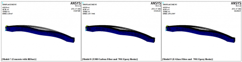
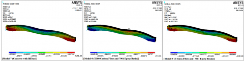
3.3 Models (7, 8, and 9)
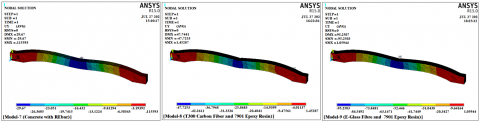
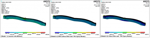
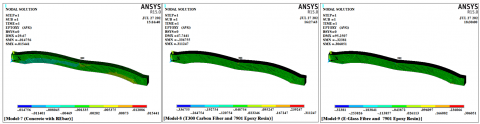
The three models (7, 8, and 9), which are composed of various composite materials but have the same geometric design, were tested using the ANSYS 15.0 program, and the Figures 53-65 show the outcomes. The results of the deflection (δ) for these models are shown in Figure 53, and the results show that the deflection values for the three models are, as is abundantly obvious $\left(\delta_7=29.67 \mathrm{~mm}, \delta_8=47.7441 \mathrm{~mm}\right.$, and $\left.\delta_9=95.2507 \mathrm{~mm}\right)$. The results of the component of the displacement in a direction (x), for these models are shown in Figure 54, The displacement outcomes are shown in the figure as follows, $\begin{aligned} & \left(\mathrm{Ux}_7=-4.034 \text { to } 4.0626 \mathrm{~mm}, \mathrm{Ux}_8=\right. \left.-3.9636 \text { to } 5.175 \mathrm{~mm}, \text { and } U x_9=-10.0258 \text { to } 9.4659 \mathrm{~mm}\right) .\end{aligned}$ Figure 55 shows the models' results for the component of displacement in a direction (y), the figure shows that the maximum results' values are, $\begin{aligned} & \left(\mathrm{Uy}_7=29.67 \mathrm{~mm}, \mathrm{Uy}_8=47.7441 \mathrm{~mm}, \text { and } \mathrm{Uy}_9=\right. 95.2503 \mathrm{~mm}) .\end{aligned}$ Figure 56 shows the components of these models' displacements in a direction (z), according to the figure, displacement values might be either positive or negative are $\begin{aligned} & \left(\mathrm{Uz}_7=-0.0594 \text { to } 0.0094 \mathrm{~mm}, \mathrm{Uz}_8=\right. \left.-0.0666 \text { to } 0.2114 \mathrm{~mm} \text {, and } \mathrm{Uz}_9=-0.1162 \text { to } 0.0048 \mathrm{~mm}\right)\end{aligned}$. The results of the normal stress (σx) for these models are shown in Figure 57, the outcomes of this stresses show the values $\begin{aligned} & \quad\left(\sigma_{x_7}=-2115.99 \text { to } 811.667 \mathrm{MPa}, \sigma_{x_8}=\right. -6259.01 \text { to } 1752.3 \mathrm{MPa} \text {, and } \sigma_{x_9}=-3071.03 \text { to } 863.097 \mathrm{MPa}) .\end{aligned}$ The results of the typical stress (σy), as shown Figure 58, the figure displays the effects of this stress for several models, with values ranging from $\begin{aligned} & \left(\sigma_{y_7}=-1915.14 \text { to } 384.78 \mathrm{MPa}, \sigma_{y_8}=\right.-2069.49 \text { to } 692.133 \mathrm{MPa}, \text { and } \sigma_{y_9}=-1498.68 \text { to } 210.28 \mathrm{MPa}) .\end{aligned}$ The results of the shear stress (τxy), for these models, are shown in Figure 59, the figure demonstrates that the shear stresses values range from $\begin{aligned} & \left(\tau_{x y_7}=-1061.82 \text { to } 1058.43 \mathrm{MPa}, \tau_{x y_8}=\right.-1331.41 \text { to } 1345.32 \mathrm{MPa} \text {, and } \tau_{x y_9}=-1261.63 \text { to } 1266.82 \mathrm{MPa}) .\end{aligned}$ The greatest stress intensity (σint.) values for the three models are shown in Figure 60 results of the stresses intensity (σint.), and they were $\begin{aligned} & \left(\sigma_{\text {int. }}=3068.31 \mathrm{MPa}, \sigma_{\text {int. }}=6604.36 \mathrm{MPa} \text {, and } \sigma_9=\right. 3746.87 \mathrm{MPa}) .\end{aligned}$ The results of the normal strain (εx), for three models, are shown in Figure 61, and the figure demonstrates that this strain's value fall within the following range $\begin{aligned} & \quad\left(\varepsilon_{x_7}=-0.0146 \text { to } 0.0070, \varepsilon_{x_8}=\right. \left.-0.0378 \text { to } 0.0250 \text {, and } \varepsilon_{x_9}=-0.0519 \text { to } 0.0184\right) .\end{aligned}$ Figure 62 shows the outcomes of these models' normal strains (εy), and the figure shows that the values of this strain range between the following values $\begin{aligned} & \left(\varepsilon_{y_7}=-0.0037 \text { to } 0.0032, \varepsilon_{y_8}=-0.0651 \text { to } 0.0399 \text {, and } \varepsilon_{y_9}=\right. -0.0903 \text { to } 0.0360) \text {. }\end{aligned}$ The results of the normal strain (εz), for three models, are shown in Figure 63, the values of the results show that the strains have values between $\begin{aligned} & \quad\left(\varepsilon_7=-0.0017 \text { to } 0.0062, \varepsilon_{z_8}=\right. \left.-0.0154 \text { to } 0.0729, \text { and } \varepsilon_{z_9}=-0.0072 \text { to } 0.0620\right) .\end{aligned}$ Figure 64 displays the results of the shear strain (εxy) for three models, this strain's value, according to the figure, fall within the following range $\begin{aligned} & \left(\varepsilon_{x y_7}=-0.0147 \text { to } 0.0154, \varepsilon_{x y_8}=\right. \left.-0.3367 \text { to } 0.3112 \text {, and } \varepsilon_{x y_9}=-0.3238 \text { to } 0.3060\right) .\end{aligned}$ The results of the models (4, 5, and 6) for the intensity strain (εxy) are shown in Figure 65, and the figure reveals that the three models' maximum strain values were $\left(\varepsilon_{\text {int. } .7}=0.0247, \varepsilon_{\text {int. } .8}=0.3387\right.$, and $\left.\varepsilon_{\text {int. } .9}=0.3252\right)$.
Figure 53. Results of the deflection (δ), for models (7, 8, and 9)
Figure 54. Results of the displacement in a direction component (Ux), for models (7, 8, and 9)
Figure 55. Results of the displacement in a direction component (Uy), for models (7, 8, and 9)
Figure 56. Results of the displacement in a direction component (Uz), for models (7, 8, and 9)
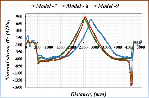
Figure 57. The results of normal stress (σx), for models (7, 8, and 9)
Figure 58. The results of normal stress (σy), for models (7, 8, and 9)
Figure 59. The results of shear stress (τxy), for models (7, 8, and 9)
Figure 60. The results of intensity stress (σint.), for models (7, 8, and 9)
Figure 61. The results of normal strain (εx), for models (7, 8, and 9)
Figure 62. The results of normal strain (εy), for models (7, 8, and 9)
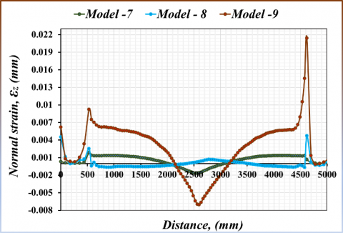
Figure 63. The results of normal strain (εz), for models (7, 8, and 9)
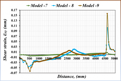
Figure 64. The results of shear strain (εxy), for models (7, 8, and 9)
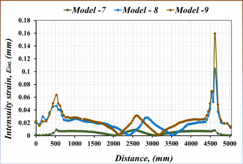
Figure 65. The results of intensity strain (εint.), for models (7, 8, and 9)
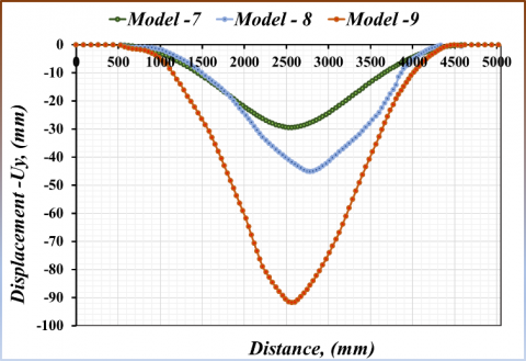
The results of using the ANSYS-15.0 program on the three models (7, 8, and 9) are shown in the Figures 66-77, which compare the deformations, stresses, and strains that the beams experience when they are fastened to the sidewalls and a load is applied to them in the middle of the surface. The path (A - A) in the figure represents the path from the beginning of the models to their end (2). The results show that: Figure 66 compares the results of various models for the relationship between displacement (Ux) and distance on a nonlinear path (C-C), and the results show that the model (M-9) had the highest displacement values, with the highest displacement positive value (9.5312 mm) being at distance and the highest displacement negative value (7.013 mm) being at distance (1,652.7 mm) (3,735 mm). The results for the nonlinear path (C-C) relationship between displacement (Uy) and distance for different models are compared in Figure 67. The figure shows that the model (M-9) experienced the most displacement, with the greatest downward displacement of (91.625 mm) happening at the distance (2,563.4 mm). Figure 68 compares the distance on a nonlinear path (C-C) and the displacement (Usum) for three different models, and the displacement (Usum) statistics in the figure indicate that the distance (2,563.4 mm) recorded the greatest values for the model (M-9), with the model's value being (91.834 mm). Figure 69 compares the results for three models for the relationship between normal stress (σx) and distance on a nonlinear path (C-C). The figure demonstrates that the model (M-9) had the highest normal stress values, the distance (4,578 mm) had the highest negative normal stress value (1,520 MPa), and the distance (2,599.8 mm) had the highest positive normal stress value (867.6 MPa). The results of various models for the connection between normal stress (σy) and distance on a nonlinear path (C-C) are compared in Figure 20, according to the figure, the model (M-7) had the highest positive normal stress (σy), and its maximal positive value was determined at a distance of (2,563.4 mm) (86.266 MPA). The maximum shear stress value (τxy) recorded for the model (M-9) is shown in Figure 71, which compares the results for various models for the relationship between shear stress (τxy) and distance along a nonlinear path (C-C), and the highest shear stresses were for the ninth model. The negative shear stress's value, which was (359.26 Mpa), was at the distance (528.86 mm), while the highest positive shear stress values were at the distance (4,620.3 mm), where they were at (811.09 MPa). Figure 72 compares the results of the relationship between distance along a nonlinear path (C-C) and stress intensity (σint.) for three different models. The data clearly demonstrate that the models (M-8, and M-9) had the highest value of stress intensity (σint.), with the first value (941.2 MPa) at the distance of (528 mm) for the ninth model, the second value (893 MPa) at the distance of (2,818.4 mm), and the third value for the ninth model at a distance of (4620.3 mm) and its value (1954.3 MPa). The results of the relationship between normal strain (εx) and distance on a nonlinear path (C-C) for three models are compared in Figure 73. The figure shows that the model (M-9) had values of the largest strain (εx), with the greatest positive strain measurements being (0.0175) and at a distance of (0.0175 mm), and the highest negative strain value being recorded at a distance of (4,578 mm) and its value being (0.0428). Figure 74 compares the findings for different models for the relationship between normal strain (εy) and distance on a nonlinear path (C-C). The figure shows that the model (M-8) recorded the highest strain value, and the normal strain value was (0.0428) at the distance (4,535.7 mm). Figure 75 compares the results for three models' normal strain (εz) and distance on a nonlinear path (C-C) relationship. The results show that the ninth model, when viewed from a distance (2,599.8 mm), had the maximum negative strain, with a value of (0.007), while the maximum positive strain, with a value of (0.0214) at the distance (4,620.3 mm). Figure 76 Compare the results of the relationship between shear strain (εxy) and distance on a nonlinear path (C-C) for these three models and the data in the figure. The ninth model had the highest shear strain (εxy), and its maximum negative shear strain value was (0.0634) at a distance (528.8 mm), in contrast to the highest positive shear strain measurement (0.1569), which was at a distance of (4,620.3 mm). For the models (7, 8, and 9), Figure 77 compares the results of the association between distance on a nonlinear path (C-C) and intensity strain (εint.). The figure shows that the ninth model had the highest strain intensity values, with its value (0.1593) at a distance (4,620.3 mm).
Figure 66. Compare the results of the relationship between displacement (Ux) and distance on a nonlinear path (C-C), for models (7, 8, and 9)
Figure 67. Compare the results of the relationship between displacement (Uy) and distance on a nonlinear path (C-C), for models (7, 8, and 9)
Figure 68. Compare the results of the relationship between displacement (Usum) and distance on a nonlinear path (C-C), for models (7, 8, and 9)
Figure 69. Compare the results of the relationship between normal stress (σx) and distance on a nonlinear path (C-C), for models (7, 8, and 9)
Figure 70. Compare the results of the relationship between normal stress (σy) and distance on a nonlinear path (C-C), for models (7, 8, and 9)
Figure 71. Compare the results of the relationship between shear stress (τxy) and distance on a nonlinear path (C-C), for models (7, 8, and 9)
Figure 72. Compare the results of the relationship between stress intensity (σint.) and distance on a nonlinear path (C-C), for models (7, 8, and 9)
Figure 73. Compare the results of the relationship between normal strain (εx) and distance on a nonlinear path (C-C), for models (7, 8, and 9)
Figure 74. Compare the results of the relationship between normal strain (εy) and distance on a nonlinear path (C-C), for models (7, 8, and 9)
Figure 75. Compare the results of the relationship between normal strain (εz) and distance on a nonlinear path (C-C), for models (7, 8, and 9)
Figure 76. Compare the results of the relationship between shear strain (εxy) and distance on a nonlinear path (C-C), for models (7, 8, and 9)
Figure 77. Compare the results of the relationship between intensity strain (εint.) and distance on a nonlinear path (C-C), for models (7, 8, and 9)
The research of several composite materials that are shaped like beams of various shapes is presented in this work. by testing the strains, stresses, and deformations that these various beams experience when subjected to a certain load. The study also focused on the comparison between the results obtained, and the following was concluded from the analysis of the results:
The data analysis findings demonstrate that the model (M-6) had the largest deflection value, and its value (381.75 mm), while the model (M-7) and its value (29.67 mm) had the least deflection. The cause of this is that ductile failures occur far less frequently in pressure-controlled columns and beams. As an illustration, failure of the crushing kind in a shaft typically happens very quickly and without prior notice. Collars are used to increase safety since they restrict the movement of the crushed aggregate.
According to the study of the data, the nonlinear models (M-4, M-5, M-6, M-7, M-8, and M-9), have higher normal stresses (σx, σy, and σz) in the locations where there are curves, they have significant stress levels, but the linear models (M-1, M-2, M-3) such stresses don't exist. This is caused by the buildup of stresses in the regions where there are bends.
It is evident from the analysis of the findings that there are hardly any shear stresses (τxz, and τyz) in any of the models. While there are significant shear stresses (τxy) of this type in the non-linear models (M-4, M-5, M-6, M-7, M-8, and M-9), these stresses are concentrated in the model's curved regions. Whereas in the eighth model, the maximum value of negative shear stress values at point (786.66 MPa, 776.92 mm), while the ninth model's point (811.09 MPa, 4620.3) had the highest positive shear stress. This is because shear stresses develop where there are bends, but not in straight models, which are not exposed to shear stresses from vertical loading.
A thorough analysis of the data reveals that stress intensity (σint.) exists in several locations across the models, including their beginnings, middles, and ends as well as in their curved portions. In the second model, the two points ((3,950 MPa, 0 mm) & (3,950 MPa, 5,000 mm)) had the highest values of stress intensity (σint.). The reason for this is that the stress concentration increases in the curved areas, and when designing, this must be taken into account, and the design depends on the stresses in the curved areas.
According to the data, the normal strains (εx, εy and εz) in the linear models (1, 2, and 3) have high values at the start, middle, and end of the models, while the normal strains (εx, εy and εz) are distributed differently in nonlinear models (M-4, M-5, M-6, M-7, M-8, and M-9), particularly in curvilinear regions where they have significant strain values. This shows that it is possible to reduce the strains at the beginning, middle and end of the straight models, by changing them with other curved models to reduce the strains in the middle, beginning and end of the models to other controlled areas during the design.
The findings demonstrate that shear stresses (εxy) in linear models (1, 2, and 3) occur at the start and end of the models, whereas shear strains in non-linear models (M-4, M-5, M-6, M-7, M-8, and M-9) in places where there are curves. This shows that the shear strains are concentrated in the areas of curvature and other curved areas in the curved and non-rectilinear models as opposed to the straight ones.
The findings indicate that the beginning, middle, and ends of the linear models (1, 2, and 3) exhibit intensity strains (εint.), but the non-linear models (M-4, M-5, M-6, M-7, M-8, and M-9) exhibit intensity strains in the areas around the curves and middle models. This indicates that the strain concentrations in the curved and non-rectangular models occur in regions different from the strains that occur in the straight models.
In future studies, we suggest using different forces such as (20 MN, 30 MN, ........) to simulate different working conditions and reveal the effect of forces on the models, as well as another study using different sizes and the effect of the size of the model on the resistance of different materials, as well as experimental models can be built, tested and compared with the results obtained.
The Ministry of Higher Education and Scientific Research of the Republic of Iraq funded the Engineering Science Research Program through the Northern Technical University/Technical Institute of Mosul, which supported this study. (No. 00333- 2022).
[1] Shalall, M.A. (2017). Nonlinear analysis of continuous composite beam by finite element method. Journal of Engineering and Development, 9(2): 54-69.
[2] Yu, W.B. (2002). Variational asymptotic modeling of composite dimensionally reducible structures. Ph.D. Thesis, Aerospace Engineering, Georgia Institute of Technology: 1-8.
[3] Pai, P.J., Nayfeh, A.H. (1992). A nonlinear composite beam theory. Nonlinear Dynamics Journal, 3(4): 273-303. https://doi.org/10.1007/BF00045486
[4] Yu, W.B., Blair, M. (2012). GEBT: A general-purpose nonlinear analysis tool for composite beams. Composite Structures Journal, 94(9): 2677-2689. https://doi.org/10.1016/j.compstruct.2012.04.007
[5] Weinberg, M. (1987). Shear testing of neat thermoplastic resins and their unidi 315 rectional figureite composites. Composites, 18(5): 386-392. https://doi.org/10.1016/0010-4361(87)90363-6
[6] Jiang, F., Deo, A., Yu, W.B. (2018). A composite beam theory for modeling nonlinear shear behavior. Engineering Structures Journal, 155: 73-90. https://doi.org/10.1016/j.engstruct.2017.10.051
[7] Karakuzu, R., Icten, B.M., Tekinsen, O. (2010). Failure behavior of composite laminates with multi-pin loaded holes. Journal of Reinforced Plastics and Composites, 29(2): 247-253. https://doi.org/10.1177/0731684408097758
[8] Chang, F.K., Chang, K.Y. (1987). A progressive damage model for laminated composites containing stress concentrations. Journal of Composite Materials, 21(9): 834-855. https://doi.org/10.1177/002199838702100904
[9] Jiang, F., Yu, W. (2015). Nonlinear variational asymptotic sectional analysis of hyperelastic beams. AIAA Journal, 54(2): 679-690. https://doi.org/10.2514/1.J054334
[10] Lee, C.S., Lee, J.M. (2015). A study on the evaluation of fiber and matrix failures for laminated composites using hashin·puck failure criteria. Journal of the Society of Naval Architects of Korea, 52(2): 143-152. https://doi.org/10.3744/SNAK.2015.52.2.143
[11] Donadon, M.V., Iannucci, L., Falzon, B.G., Hodgkinson, J.M., de Almeida, S.F.M. (2008). A progressive failure model for composite laminates subjected to low velocity impact damage. Computers & Structures, 86(11-12): 1232-1252. https://doi.org/10.1016/j.compstruc.2007.11.004
[12] Lomakin, E.V., Fedulov, B.N. (2015). Nonlinear anisotropic elasticity for laminate composites. Meccanica, 50(6): 1527-1535. https://doi.org/10.1007/s11012-015-0104-5
[13] Žarković, D. (2022). Matrix 3d software for linear and non-linear structural analysis and design. Materials: Conference Contemporary Civil Engineering Practice, Serbia. https://www.researchgate.net/publication/361307277
[14] Grassl, P., Xenos, D., Nyström, U., Rempling, R., Gylltoft, K. (2013). CDPM2: A damage-plasticity approach to modelling the failure of concrete. International Journal of Solids and Structures, 50(24): 3805-3816. https://doi.org/10.1016/j.ijsolstr.2013.07.008
[15] Karash, E.T., Sultan, J.N., Najem, M.K. (2021). The difference in the wall thickness of the helicopter structure are made of composite materials with another made of steel. Mathematical Modelling of Engineering Problems 9(2): 313-324. https://doi.org/10.18280/mmep.090204
[16] Najim, M., Sultan, J., Karash, E. (2020). Comparison of the resistance of solid shell of composite materials with other solid metal Materials. In: IMDC-SDSP 2020, pp. 28-30. https://doi.org/10.4108/eai.28-6-2020.2298518
[17] Žarković, D., Jovanović, Đ., Vukobratović, V., Brujić, Z. (2019). Convergence improvement in computation of strain-softening solids by the arc-length method. Finite Elements in Analysis and Design, 164: 55-68. https://doi.org/10.1016/j.finel.2019.06.005
[18] Karash, E.T., Alsttar Sediqer, T.A., Elias Kassim, M.T. (2021). A comparison between a solid block made of concrete and others made of different composite materials. Revue des Composites et des Matériaux Avancés, 31(6): 341-347. https://doi.org/10.18280/RCMA.310605
[19] Karash, E.T. (2011). Modelling of unilateral contact of metal and fiberglass shells. Applied Mechanics and Materials Journal, 87: 206-208. https://doi.org/10.4028/www.scientific.net/AMM.87.20
[20] Karash, E.T. (2017). The study contacts bending stress two-layer plates from fiberglass with interfacial defects of structure. Agricultural Research & Technology, 12(1): 555834. https://doi.org/10.19080/ARTOAJ.2017.12.555834
[21] Bernuzzi, C., Simoncelli, M., Venezia, M. (2017). Performance of mono-symmetric upright pallet racks under slab deflections. Journal of Constructional Steel Research, 128: 672-686. https://doi.org/10.1016/j.jcsr.2016.10.004
[22] Najem, M.K., Karash, E.T., Sultan, J.N. (2021). The amount of excess weight from the design of an armored vehicle body by using composite materials instead of steel. Revue des Composites et des Matériaux Avancés-Journal of Composite and Advanced Materials, 32(1): 1-10. https://doi.org/10.18280/rcma.320101
[23] Avalon, S.C., Donaldson, S.L. (2010). Strength of composite angle brackets with multiple geometries and nanofiber-enhanced resins. Journal of Composite Materials, 45(9): 1017-1030. https://doi.org/10.1177/0021998310381538
[24] Vershchaka, M., Zhigiliy, D.A., Karash, E.T. (2012). The experimental model of the pipe of a composite material under the effect of internal pressure. International Journal of Science and Engineering Investigations, 1(5): 1-4.
[25] Ranz, D., Cuartero, J., Miravete, A., Miralbes, R. (2016). Experimental research into interlaminar tensile strength of carbon/epoxy laminated curved beams. Composite Structures Journal, 164: 1-15. https://doi.org/10.1016/j.compstruct.2016.12.010
[26] Vereshaka, S.M., Karash, T.E. (2021). Experimental model of the semicircular laminated composite curved bars. International Journal of Structronics & Mechatronics, 1(1): 67-73. https://doi.org/10.18280/RCMA.310605
[27] Palanim, G.S., Rajasekaran, S. (1992). Finite element analysis of thin-walled curved beams made of composites. Journal of Structural Engineering, 118(8): 2039-2062. https://doi.org/10.1061/(ASCE)0733-9445(1992)118:8(2039)
[28] Cortínez, V.H., Piovan, M.T., Machado, S. (2001). DQM vibration analysis of composites thin-walled curved beams. Journal of Sound and Vibration, 246(3): 551-555. https://doi.org/ 10.1006/jsvi.2001.3600
[29] Liu, X., Tang, T., Yu, W.B., Byron Pipes, R. (2018). Multiscale modeling of viscoelastic behaviors of textile composites using mechanics of structure genome. American Institute of Aeronautics and Astronautics. https://doi.org/10.2514/6.2018-0899
[30] Hao, W.F., Ge, D.Y., Ma, Y., Yao, X.F., Shi, Y. (2012), Experimental investigation on deformation and strength of carbon/epoxy laminated curved beams. Polymer Testing Jurnal, 31(4): 520-526. https://doi.org/10.1016/j.polymertesting.2012.02.003
[31] Raju, R. (2014). Delamination damage analysis of curved composites subjected to compressive load using cohesive zone modelling. Conference: First world Conference on Fracture and Damage Mechanics (FRACTURE-2014), pp. 36-45. https://www.researchgate.net/publication/281624445.
[32] Kaafi, P., Amiri, G.G. (2020). Investigation of the progressive collapse potential in steel buildings with composite floor system. Journal of Structural Engineering and Geotechnics, 10(2): 169-179. https://www.researchgate.net/publication/355080838.
[33] Seshavenkat Naidu, B., Krovvidi, S. (2021). Fabrication of E-glass fibre based composite material with induced particulate additives. IOP Conference Series: Materials Science and Engineering, 1033: 012075. https://doi.org/10.1088/1757-899X/1033/1/012075