Duc Ngoc Nguyen*![]() | Tuan Anh Nguyen
| Tuan Anh Nguyen![]()
© 2023 IIETA. This article is published by IIETA and is licensed under the CC BY 4.0 license (http://creativecommons.org/licenses/by/4.0/).
OPEN ACCESS
The content done in this article is the problems with the vehicle's rollover dynamics when steering. In this article, a complex dynamics model is established, which fully includes the influence of external factors. This complex model combines the models of spatial dynamics (7 DOFs - degrees of freedom), nonlinear double-track dynamics (3 DOFs), and the Pacejka nonlinear tire model. The simulation and calculation process are done by the MATLAB-Simulink application. The input parameters of the oscillation problem include the steering angle and velocity of the vehicle. These values are adjusted based on three specific cases and three situations. The output values that can evaluate the vehicle's oscillations include the roll angle, vertical force, and a trajectory of the vehicle. The results of the article have shown the oscillation of an automobile in all investigated cases. As a consequence of these findings, the vehicle's oscillation is greatest when the speed and steering angle reach their maximum values. When the vehicle was steered in "Fishhook" mode, the vehicle rolled over at v2 = 70 (km/h) and v3 = 80 (km/h). The limited roll angle corresponding to these two situations are 9.41˚ and 9.26˚, respectively. Under the influence of the tire's nonlinear deformation, the vehicle's motion trajectory also changes greatly. This model should be used for research problems involving motion trajectories and vehicle rollover.
vehicle dynamic, complex model, simulation and model, oscillation
Vehicle dynamics is a fairly common topic. It has been studied for many years. The level of research in this area has changed over time. This field usually involves the study of oscillations and movements of the vehicle when going straight or steering. Besides, studies of suspension system vibration can also be considered [1]. The input parameters of the problem of vehicle dynamics usually include the speed of a vehicle, the steering angle, the roughness of the road surface, etc. Output values can be mentioned as roll angle, yaw angle, vertical force, longitudinal force, lateral force, acceleration and displacement of the sprung mass, etc. [2]. Depending on the problem, there will be specific content.
An integrated dynamics model is often utilized in order to simulate the vehicle's oscillations when steering. This model will include an oscillation model of the vehicle body, a model of motion, and a tire model. There are some combinations of vehicle dynamics models. For the oscillation model of the vehicle body, researchers often use a half dynamics model [3]. This model is quite simple; it only includes 4 degrees of freedom (DOFs) [4]. If seats are included, a number of DOFs of this model can be increased [5]. The half-dynamics model usually only includes the influence of pitch angle or roll angle [6, 7]. Spatial dynamics models can include both of these influences [8]. According to Nguyen, spatial dynamics models usually have 7 degrees of freedom [9, 10]. For large vehicles, a number of DOFs can be more [11]. When the vehicle is moving, single-track or double-track dynamics models can be used [12, 13]. The linear single-track dynamics model is much simpler than the others. According to Gao et al. [14], two wheels on an axle can be combined. This model includes only 2 degrees of freedom [15]. In this model, many effects were ignored [16]. In contrast, the nonlinear double-track dynamics model will consider all influences of the wheels [17]. In this model, the steering angles of the wheels can be the same or different [18]. Unknowns in the motion model are usually lateral force Fy, longitudinal force Fx, etc. These values can be calculated according to the tire model. The linear tire model is the simplest [19]. However, its accuracy is not high. The linear tire model is only valid when an automobile is traveling at a low velocity and the steering angle is small [20]. The linear tire model can be incorporated with a linear single-track or nonlinear double-track dynamics model [21]. To be able to accurately assess the impact of the tire, several modern tire models should be used, such as Pacejka, Ammon, Burckhardt, Empirical, Dugoff, Brush, etc. [22-25]. In addition, the combination of simulation software and intelligent algorithms is also recommended to be able to determine the tire influence [26-28].
This article aims to establish a model of complex dynamics to simulate vehicle oscillations. This model includes external influences when an automobile is travelling on the road. This combines a spatial dynamics model (7 DOFs) and a nonlinear double-track model (3 DOFs). The 7 DOFs spatial dynamics model provides a complete description of vehicle oscillations, which include vertical, roll, and pitch displacements. Meanwhile, the 3 DOFs nonlinear double-track dynamics model describes the influence of all four wheels on the car's motion (including longitudinal, lateral, and yaw movements). In addition, the nonlinear motion model describes the influence of other external factors, such as lateral and longitudinal wind forces (if applicable). Besides, the interaction between the wheel and the road surface is determined by the Pacejka nonlinear tire model. This tire model considers the tire's elastic deformation during steering, which involves varying the tire lateral force values. Compared with conventional linear models (such as the half model, which is combined with the linear single-track model and the linear tire model), the model of the complex dynamics that is designed in this study helps to describe the oscillations more wholly and accurately. This model is rarely used because of its computational complexity. The process of numerical simulation and calculation is done by MATLAB software with specific cases. The main content of this article includes of four sections, including introduction section, complex dynamics model section, simulation and discussions section, and conclusion section.
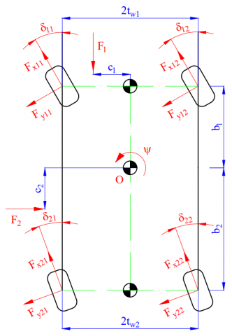
The complex dynamics model consists of three components: the fully dynamics model, the nonlinear double-track model, and the nonlinear tire model. The fully dynamics model with 7 DOFs is shown in Figure 1. In this model, a vehicle body is called a sprung mass. Components below a suspension system are known as "unsprung mass". Using the separation method, the sprung mass performs three movements corresponding to three DOFs, including vertical displacement, roll, and pitch. Meanwhile, the four unsprung masses only perform four vertical displacements, corresponding to four DOFs. The tire's damping component is ignored because its damping capacity is much smaller than the suspension dampers. The equations describing vehicle's oscillations when steering is pointed as below:
Figure 1. Model of the fully dynamics with 7 DOFs
${{F}_{ims}}=\sum\limits_{i,j=1}^{2}{\left( {{F}_{Kij}}+{{F}_{Cij}} \right)}$ (1)
$\begin{aligned} & M_\phi=\sum_{i, j=1}^2\left[(-1)^{j-1}\left(F_{K i j}+F_{C i j}\right) t_{w i}\right] \\ & +\left\{g \sin \phi+\left[\dot{v}_y+(\dot{\beta}+\dot{\psi}) v_x\right] \cos \phi\right\} m_s h_\phi\end{aligned}$ (2)
${{M}_{\theta }}=\sum\limits_{i,j=1}^{2}{{{\left( -1 \right)}^{i-1}}\left( {{F}_{Kij}}+{{F}_{Cij}} \right){{b}_{i}}}$ (3)
${{F}_{imuij}}={{F}_{KTij}}-{{F}_{Kij}}-{{F}_{Cij}}$ (4)
where:
${{F}_{ims}}={{m}_{s}}{{\ddot{z}}_{s}}$ (5)
${{F}_{imuij}}={{m}_{uij}}{{\ddot{z}}_{uij}}$ (6)
${{F}_{Kij}}={{K}_{ij}}\left[ {{z}_{s}}-{{z}_{uij}}+{{\left( -1 \right)}^{j+1}}{{t}_{wi}}\phi +{{\left( -1 \right)}^{i+1}}{{b}_{i}}\theta \right]$ (7)
${{F}_{Cij}}={{C}_{ij}}\left[ {{{\dot{z}}}_{s}}-{{{\dot{z}}}_{uij}}+{{\left( -1 \right)}^{j+1}}{{t}_{wi}}\dot{\phi }+{{\left( -1 \right)}^{i+1}}{{b}_{i}}\dot{\theta } \right]$ (8)
${{F}_{KTij}}={{K}_{Tij}}\left( {{z}_{rij}}-{{z}_{uij}} \right)$ (9)
${{M}_{\phi }}=\left( {{J}_{\phi }}+{{m}_{s}}h_{\phi }^{2} \right)\ddot{\phi }$ (10)
${{M}_{\theta }}=\left( {{J}_{\theta }}+{{m}_{s}}h_{\theta }^{2} \right)\ddot{\theta }$ (11)
The components of the longitudinal velocity vx, lateral velocity vy, and yaw angle $\psi$ are determined by a nonlinear double-track dynamics model (Figure 2). This model performs three movements, including longitudinal x, lateral y, and yaw $\psi$, corresponding to three degrees of freedom.
Figure 2. Model of the nonlinear double-track dynamics
${{F}_{ix}}=\sum\limits_{i,j=1}^{2}{\left( {{F}_{xij}}cos{{\delta }_{ij}}-{{F}_{yij}}sin{{\delta }_{ij}} \right)}-{{F}_{1}}+{{F}_{cex}}$ (12)
${{F}_{iy}}=\sum\limits_{i,j=1}^{2}{\left( {{F}_{xij}}sin{{\delta }_{ij}}+{{F}_{yij}}cos{{\delta }_{ij}} \right)}-{{F}_{2}}-{{F}_{cey}}$ (13)
$M_\psi=\sum_{i, j=1}^2\left[\begin{array}{l}(-1)^j\left(F_{x i j} \cos \delta_{i j}-F_{y i j} \sin \delta_{i j}\right) t_{\mathrm{w} i} \\ +(-1)^{i+1}\left(F_{x i j} \sin \delta_{i j}+F_{y i j} \cos \delta_{i j}\right) b_i \\ +F_i c_i-M_{z i j}\end{array}\right]$ (14)
where:
${{F}_{ix}}=\left( {{m}_{s}}+\sum\limits_{i,j=1}^{2}{{{m}_{ij}}} \right){{\dot{v}}_{x}}$ (15)
${{F}_{iy}}=\left( {{m}_{s}}+\sum\limits_{i,j=1}^{2}{{{m}_{ij}}} \right){{\dot{v}}_{y}}$ (16)
${{F}_{cex}}=\left( {{m}_{s}}+\sum\limits_{i,j=1}^{2}{{{m}_{ij}}} \right)\left( \dot{\beta }+\dot{\psi } \right){{v}_{y}}$ (17)
${{F}_{cey}}=\left( {{m}_{s}}+\sum\limits_{i,j=1}^{2}{{{m}_{ij}}} \right)\left( \dot{\beta }+\dot{\psi } \right){{v}_{x}}$ (18)
${{M}_{\psi }}={{J}_{\psi }}\ddot{\psi }$ (19)
$\beta =arctan\frac{{{v}_{y}}}{{{v}_{x}}}$ (20)
The forces and moments at the wheel, including longitudinal force Fx, moment Mz, and lateral force Fy are calculated by a tire model. In this article, the Pacejka tire model is utilized.
Longitudinal force Fx:
${{F}_{x}}={{D}_{x}}sin\left[ {{C}_{x}}artan\left( {{B}_{x}}{{\kappa }_{x}} \right) \right]$ (21)
where:
${{\kappa }_{x}}=\left( 1-{{E}_{x}} \right)\lambda +\frac{{{E}_{x}}}{{{B}_{x}}}arctan\left( {{B}_{x}}\lambda \right)$ (22)
${{C}_{x}}=1.65$ (23)
${{D}_{x}}={{a}_{1}}F_{z}^{2}+{{a}_{2}}{{F}_{z}}$ (24)
$BC{{D}_{x}}=\frac{{{a}_{3}}F_{z}^{2}+{{a}_{4}}{{F}_{z}}}{{{e}^{{{a}_{5}}{{F}_{z}}}}}$ (25)
${{B}_{x}}=\frac{BC{{D}_{x}}}{{{C}_{x}}{{D}_{x}}}$ (26)
${{E}_{x}}={{a}_{6}}F_{z}^{2}+{{a}_{7}}{{F}_{z}}+{{a}_{8}}$ (27)
Lateral force Fy:
${{F}_{y}}={{D}_{y}}sin\left[ {{C}_{y}}artan\left( {{B}_{y}}{{\kappa }_{y}} \right) \right]+{{S}_{vy}}$ (28)
where:
${{\kappa }_{y}}=\left( 1-{{E}_{y}} \right)\left( \alpha +{{S}_{hy}} \right)+\frac{{{E}_{y}}}{{{B}_{y}}}arctan\left[ {{B}_{y}}\left( \alpha +{{S}_{hy}} \right) \right]$ (29)
${{C}_{y}}=1.30$ (30)
${{D}_{y}}={{a}_{1}}F_{z}^{2}+{{a}_{2}}{{F}_{z}}$ (31)
$BC{{D}_{y}}={{a}_{3}}sin\left[ {{a}_{4}}artan\left( {{a}_{5}}{{F}_{z}} \right) \right]$ (32)
${{B}_{y}}=\frac{BC{{D}_{y}}}{{{C}_{y}}{{D}_{y}}}$ (33)
${{E}_{y}}={{a}_{6}}F_{z}^{2}+{{a}_{7}}{{F}_{z}}+{{a}_{8}}$ (34)
${{S}_{hy}}={{a}_{9}}\gamma $ (35)
${{S}_{vy}}=\left( {{a}_{10}}F_{z}^{2}+{{a}_{11}}{{F}_{z}} \right)\gamma $ (36)
Aligning moment Mz:
${{M}_{z}}={{D}_{z}}sin\left[ {{C}_{z}}artan\left( {{B}_{z}}{{\kappa }_{z}} \right) \right]+{{S}_{vz}}$ (37)
where:
${{\kappa }_{z}}=\left( 1-{{E}_{z}} \right)\left( \alpha +{{S}_{hz}} \right)+\frac{{{E}_{z}}}{{{B}_{z}}}arctan\left[ {{B}_{z}}\left( \alpha +{{S}_{hz}} \right) \right]$ (38)
${{C}_{z}}=2.40$ (39)
${{D}_{z}}={{a}_{1}}F_{z}^{2}+{{a}_{2}}{{F}_{z}}$ (40)
$BC{{D}_{z}}=\frac{{{a}_{3}}F_{z}^{2}+{{a}_{4}}{{F}_{z}}}{{{e}^{{{a}_{5}}{{F}_{z}}}}}$ (41)
${{B}_{z}}=\frac{BC{{D}_{z}}}{{{C}_{z}}{{D}_{z}}}$ (42)
${{E}_{z}}={{a}_{6}}F_{z}^{2}+{{a}_{7}}{{F}_{z}}+{{a}_{8}}$ (43)
${{S}_{hz}}={{a}_{9}}\gamma $ (44)
${{S}_{vz}}=\left( {{a}_{10}}F_{z}^{2}+{{a}_{11}}{{F}_{z}} \right)\gamma $ (45)
Figure 3. Slip ratio and longitudinal force
Figure 4. Slip angle and lateral force
Based on the established tire model, the dependence between slip ratio and longitudinal force; the slip angle and lateral force is shown in Figure 3 and Figure 4.
3.1 Simulation
To simulate vehicle dynamics when steering, some vehicle motion conditions should be defined in advance. There are three steering angles used (Figure 5), including single-lane change, J-turn, and fishhook, corresponding to three cases. These three typical types of steering often occur when drivers use cars. Besides, these types of steering are also often used in simulation problems related to vehicle rollover oscillations. In each case, the speed of the vehicle will change to the following values: v1 = 60 (km/h), v2 = 70 (km/h), and v3 = 80 (km/h). The simulation and calculation are done by MATLAB application. The outputs of this problem include the vertical force, roll angle, and the trajectory of a vehicle.
The automobile's parameters are referred to in Table 1.
Figure 5. Steering angle (a – single lane change; b – J-turn; c – fishhook)
Table 1. The vehicle parameters
|
Symbol |
Description |
Value |
Unit |
|
ms |
Sprung mass |
1850 |
kg |
|
mu |
Unsprung mass |
40 |
kg |
|
bi |
Distance from the center of gravity to axle |
1.25/1.64 |
m |
|
twi |
Half of the track width |
0.730/0.725 |
m |
|
$\mathrm{J}_\phi$ |
The moment of inertia of the roll-axis |
710 |
kgm2 |
|
$\mathrm{J}_\theta$ |
The moment of inertia of the pitch-axis |
2795 |
kgm2 |
|
$\mathrm{J}_\psi$ |
The moment of inertia of the yaw-axis |
2710 |
kgm2 |
|
$\mathrm{h}_\theta$ |
Distance from the center of gravity to roll-axis |
0.53 |
M |
|
g |
Gravitational acceleration |
9.81 |
m/s2 |
|
Ci |
Damping coefficient |
3150/3080 |
Ns/m |
|
Ki |
Spring coefficient |
38500/37300 |
N/m |
|
KTi |
Tire coefficient |
17500/17500 |
N/m |
3.2 Results
Case 1: Single-lane change
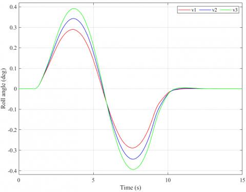
Automobiles often utilize the "single-lane change" steering angle when changing lanes. Because the distance between the two lanes is small, a steering angle used is also very small. A change of the roll angle with simulation time is illustrated in Figure 6. These values are very small and do not affect the stability of an automobile. Because the vehicle oscillation is small, the change in dynamics force at wheels is also not large (Figure 7). If the velocity is smaller, the change will be smaller. When the steering wheel returns to its original position, the change in these values is also gone.
Figure 6. Roll angle – Case 1
Figure 7. Vertical force – Case 1
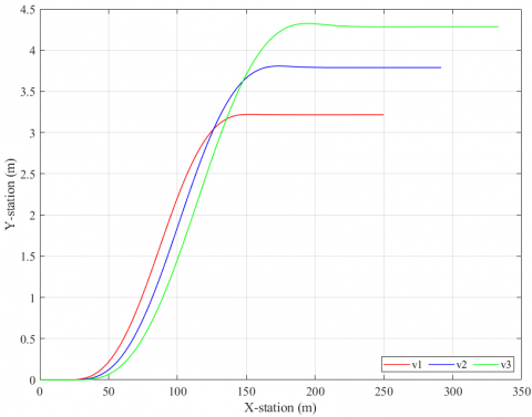
The vehicle’s trajectory in motion is shown in Figure 8. When the speed is greater, the trajectory of the vehicle's motion will also be larger (both longitudinally and laterally). In this case, the results obtained from the simulation of the nonlinear model are similar to those obtained from conventional linear models. Larger steering angles are needed to show the difference.
Figure 8. The trajectory of the vehicle – Case 1
Case 2: J-turn
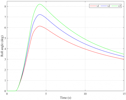
A "J-turn" steering angle is often utilized when an automobile enters the roundabout. The value of the steering angle will be increased by a certain amount. After that, this value will be kept for a period of time. Figure 9 illustrates a change in the roll angle corresponding to three velocity values. According to these results, a maximum roll angle value is 8.21˚ at a velocity of v3 = 80 (km/h). After the maximum value is reached, the magnitude of the roll angle will decrease with time. Although the steering angle remains the same, the roll angle still changes. This is caused by the nonlinear deformation of a tire. The tire's slip angle will gradually decline with time, so the value of the lateral force will also decline gradually. This results in a decreasing a vehicle roll angle. However, it is only zero once the steering angle is zero.
Figure 9. Roll angle – Case 2
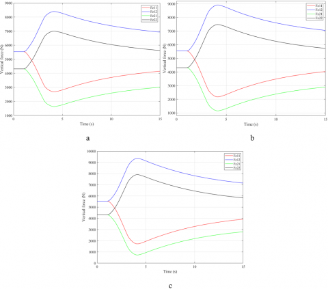
Figure 10. Vertical force – Case 2
Figure 11. The trajectory of the vehicle – Case 2
The change in the dynamics force at wheels will follow the change in a roll angle (Figure 10). This difference is greatest when an automobile is travelling at its highest speed. Then, this difference will decrease over time. In the third situation (the vehicle moves at v3), the minimum value of the dynamics force at a wheel is only 730.4 (N). This is a small value. Once this value approaches zero, the wheel can be detached from the road. At that time, a phenomenon of the rollover may occur.
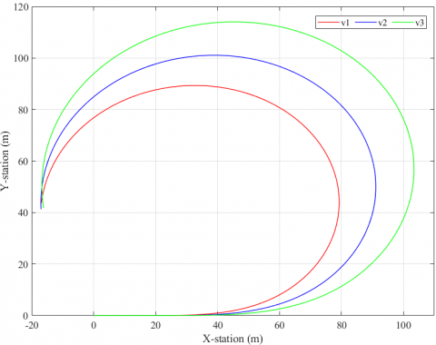
If the vehicle only uses a simple dynamics model, which includes a combination of a linear single-track dynamics model, a half-dynamics model, and a linear tire model, the vehicle's trajectory will take the form of a circle with a constant radius. In this article, a model of complex dynamics that takes into account nonlinear tire deformation is used, so the vehicle's trajectory changes nonlinearly. This trajectory has the form of a spiral curve with a decreasing radius. At the same time, the vehicle's trajectory will be longer if its velocity is greater (Figure 11).
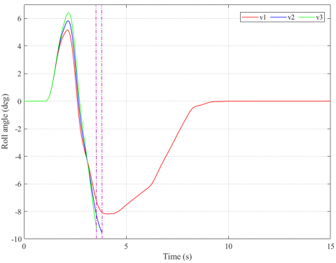
Figure 12. Roll angle – Case 3
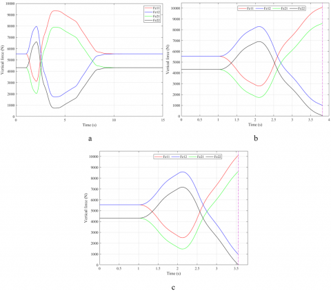
Figure 13. Vertical force – Case 3
Case 3: Fishhook
When evaluating the rollover phenomenon, the "fishhook" steering angle is often used. This type of a steering angle can cause the rollover phenomenon at high speeds. This steering angle has two phases. In the second phase, the steering acceleration and steering angle are also larger. At a velocity of v1 = 60 (km/h), the vehicle has not rolled over. The maximum roll angle value is only 8.19˚, corresponding to the minimum dynamics force value at the wheel of 751.9 (N). Once the speed is increased to v2 = 70 (km/h), the rollover occurs at time t = 3.78 (s), and the limited roll angle can achieve 9.41˚. If the speed continues to increase, v3 = 80 (km/h), the vehicle may roll over sooner. Therefore, the limited roll angle is only 9.26˚ (Figure 12).
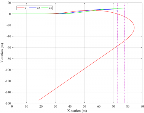
Once the vehicle rolls over, the vertical force at the wheel is reduced to zero. This is a warning sign of the rollover phenomenon (Figure 13). In this case, the vehicle's trajectory has a rather complicated form. Because of the effect of high speed and large steering angle, the nonlinear deformation of the tire will also be larger (Figure 14).
Figure 14. The trajectory of the vehicle – Case 3
This article focuses on simulating the vehicle's rollover oscillations when steering. A complex rollover dynamics model is established in this study. This combines the fully dynamics model, the nonlinear double-track dynamics model, and the nonlinear tire model. Factors affecting vehicle oscillation are fully included in this model. The simulation process is done by MATLAB software with three cases. In each case, three velocity values are used. The output values of the simulation include the roll angle, vertical force, and a trajectory of the vehicle.
Simulation results have shown the change in these values over time. Once the steering angle is larger, or the travel speed is greater, the change in value will also be larger. In the third case, the vehicle rolled over at v2 and v3. The values obtained from the simulation are completely consistent with reality. This model of complex dynamics can be used for complex antiroll and oscillation control problems. However, this study still has some disadvantages that cannot be resolved entirely, such as the parameters of the nonlinear tire model cannot be absolutely accurate, the influencing factors of the road surface and the wind have not been fully mentioned, etc. In the future, these problems should be fixed. In addition, conducting some tests on automotive dynamics is necessary to help substantiate the results of this research.
|
$\theta$ |
Pitch angle, rad |
|
$\psi$ |
Yaw angle, rad |
|
$\phi$ |
Roll angle, rad |
|
$\delta$ |
Steering angle, rad |
|
zs |
Displacement of the sprung mass, m |
|
zu |
Displacement of the unsprung mass, m |
|
zr |
Roughness on the road, m |
|
FC |
Damping force, N |
|
FK |
Spring force, N |
|
FKT |
Tire force, N |
|
Fx |
Longitudinal force, N |
|
Fy |
Lateral force, N |
|
Fz |
Vertical force, N |
|
Mz |
Aligning moment, Nm |
|
vx |
Longitudinal velocity, m/s |
|
vy |
Lateral velocity, m/s |
[1] Nguyen, T.A. (2021). Advance the efficiency of an active suspension system by the sliding mode control algorithm with five state variables. IEEE Access, 9: 164368-164378. https://doi.org/10.1109/ACCESS.2021.3134990
[2] Nguyen, T.A. (2021). New methods for calculating the impact force of the mechanical stabilizer bar on a vehicle. International Journal on Engineering Applications, 9(5): 251-257. https://doi.org/10.15866/irea.v9i5.19584
[3] Goga, V., Klucik, M. (2012). Optimization of vehicle suspension parameters with use of evolutionary computation. Procedia Engineering, 48: 174-179. https://doi.org/10.1016/j.proeng.2012.09.502
[4] Khan, M.A., Abid, M., Ahmed, N., Wadood, A., Park, H. (2020). Nonlinear control design of a half-car model using feedback linearization and an LQR controller. Applied Sciences, 10(9): 3075. https://doi.org/10.3390/app10093075
[5] Kirli, A. (2015). Design and application of an active suspension system on a 6 DOF half vehicle model. Proceedings of the 2015 XXV International Conference on Information, Communication and Automation Technologies, pp. 1-6. https://doi.org/10.1109/ICAT.2015.7340500
[6] Rideout, D.G. (2012). Simulating coupled longitudinal, pitch and bounce dynamics of trucks with flexible frames. Modern Mechanical Engineering, 2(4): 176-189. https://doi.org/10.4236/mme.2012.24023
[7] Wang, Z.F., Dong, M.M., Gu, L., Rath, J.J., Qin, Y.C., Bai, B. (2017). Influence of road excitation and steering wheel input on vehicle system dynamic responses. Applied Sciences, 7(6): 570. https://doi.org/10.3390/app7060570
[8] Setiawan, J.D., Safarudin, M., Singh, A. (2009). Modeling, simulation and validation of 14 DOF full vehicle model. Proceedings of the International Conference on Instrumentation, Communication, Information Technology, and Biomedical Engineering, pp. 1-6. https://doi.org/10.1109/ICICI-BME.2009.5417285
[9] Nguyen, T.A. (2021). Improving the stability of the passenger vehicle by using an active stabilizer bar controlled by the fuzzy method. Complexity, 2021: 6569298. https://doi.org/10.1155/2021/6569298
[10] Nguyen, T.A. (2021). Control the hydraulic stabilizer bar to improve the stability of the vehicle when steering. Mathematical Modelling of Engineering Problems, 8(2): 199-206. https://doi.org/10.18280/mmep.080205
[11] Sharma, S.K., Chouksey, M., Rawal, B.R. (2016). Numerical studies using full car model for combined primary and cabin suspension. Procedia Technology, 23: 171-178. https://doi.org/10.1016/j.protcy.2016.03.014
[12] Zhang, H., Zhang, X.J., Wang, J.M. (2014). Robust gain-scheduling energy-to-peak control of vehicle lateral dynamics stabilization. Vehicle System Dynamics: International Journal of Vehicle Mechanics and Mobility, 52(3): 309-340. https://doi.org/10.1080/00423114.2013.879190
[13] Belrzaeg, M., Ahmed, A.A., Almabrouk, A.Q., Khaleel, M.M., Ahmed, A.A., Almukhtar, M. (2021). Vehicle dynamics and tire models: An overview. World Journal of Advanced Research and Reviews, 12(1): 331-348. https://doi.org/10.30574/wjarr.2021.12.1.0524
[14] Gao, F., Hu, Q.X., Ma, J. (2021). A simplified vehicle dynamics model for motion planner designed by nonlinear model predictive control. Applied Sciences, 11(21): 9887. https://doi.org/10.3390/app11219887
[15] Miloradovic, D., Glišović, J., Stojanović, N., Grujić, I. (2019). Simulation of vehicle’s lateral dynamics using nonlinear model with real inputs. IOP Conference Series: Materials Science and Engineering, 659: 012060. https://doi.org/10.1088/1757-899X/659/1/012060
[16] Yang, S.P., Lu, Y.J., Li, S.H. (2013). An overview on vehicle dynamics. International Journal of Dynamics and Control, 1: 385-395. https://doi.org/10.1007/s40435-013-0032-y
[17] Fan, X.B., Zhao, Z.X. (2019). Vehicle dynamics modelling and electronic stability program/active front steering sliding mode integrated control. Asian Journal of Control, 21(5): 2364-2377. https://doi.org/10.1002/asjc.1822
[18] Nguyen, T.A. (2020). Establishing the dynamics model of the vehicle using the 4-wheels steering systems. Mathematical Modelling of Engineering Problems, 7(3): 436-440. https://doi.org/10.18280/mmep.070314
[19] Kissai, M., Monsuez, B., Tapus, A., Martinez, D. (2017). A new linear tire model with varying parameters. Proceedings of the 2nd IEEE International Conference on Intelligent Transportation Engineering, pp. 108-115. https://doi.org/10.1109/ICITE.2017.8056891
[20] Anh, N.T., Binh, H.T. (2020). Determining the vertical force when steering. Advances in Systems Science and Application, 20(4): 27-35. https://doi.org/10.25728/assa.2020.20.4.870
[21] Tuan, A.N., Thang, B.H. (2019). Research on dynamic vehicle model equipped active stabilizer bar. Advances in Science, Technology and Engineering Systems Journal, 4(4): 271-275. https://doi.org/10.25046/aj040434
[22] Zhang, Y., Bei, S.Y., Li, B., Jin, Y.J., Yan, H. (2018). A review of the research on the mechanical model of vehicle tires. Advances in Engineering Research, 154: 437-444.
[23] Ruzinskas, A., Sivilevicius, H. (2017). Magic formula tyre model application for a tyre-ice interaction. Procedia Engineering, 187: 335-341. https://doi.org/10.1016/j.proeng.2017.04.383
[24] Bian, M., Chen, L., Luo, Y.G., Li, K.Q. (2014). A dynamic model for tire/road friction estimation under combined longitudinal/lateral slip situation. SAE Technical Paper. https://doi.org/10.4271/2014-01-0123
[25] Svendenius, J., Wittenmark, B. (2003). Brush tire model with increased flexibility. Proceedings of the 2003 European Control Conference, pp. 1863-1868. https://doi.org/10.23919/ECC.2003.7085237
[26] Olazagoitia, J.L., Perez, J.A., Badea, F. (2020). Identification of tire model parameters with artificial neural networks. Applied Sciences, 10(24): 9110. https://doi.org/10.3390/app10249110
[27] Kanchwala, H., Viana, Í.B., Ceccoti, M., Aouf, N. (2019). Model predictive tracking controller for a high fidelity vehicle dynamics model. Proceedings of the IEEE Intelligent Transportation Systems Conference, pp. 1496-1503. https://doi.org/10.1109/ITSC.2019.8917528
[28] Vandi, G., Moro, D., Ponti, F., Parenti, R., Einaudi, G. (2013). Vehicle dynamics modeling for real-time simulation. SAE Technical Paper. https://doi.org/10.4271/2013-24-0144