Deepak Bharadwaj* | Durga Dutt
© 2022 IIETA. This article is published by IIETA and is licensed under the CC BY 4.0 license (http://creativecommons.org/licenses/by/4.0/).
OPEN ACCESS
Joint controlling is n issues in humanoid robotics. Due to large number of joint present in the humanoid robot, nonlinearity causes the problem for a smooth walk. Processor has to do a lot of computation before the execution of the operation. Due to Serial and parallel linkages of Human manipulator structure, controlling is done with the mixed mode of the operation. The Central pattern generator (CPG) controller architecture were adopted for the such type of operation. CPG controller system interact with the environment and generates the task for the joint using the trajectory control. A simple master-slave control architecture was implemented for the controlling of the lower body of a humanoid robot trajectory. The nonlinearity was minimized by selecting the popper gear ratio. The stiffness and damping designed based on the natural frequency of the system. The controller design was optimized at damping factor 1. The structural oscillations were minimized due to enhance the gain of the controller. The stability of joint control enhance.
control architecture, computed control torque, gain
Humanoid robot has more number of joint and links. Due to presence of serial and parallel linkages, system becomes complicated to control. The processor has to do the several computations before to the actuation of the joint. Several degrees of freedom in the humanoid system make the system unstable and unable to do the desired task in the dynamic environment [1]. The control system of the humanoid robot is separated into different modules. Each part has its software and hardware module. The first layer of cognitive control architecture consists of sensors and motors and its need not require any access from the system knowledge database. The data coming from the joint position sensor, force sensor, and tactile artificial sensitive skin passed to the middle layer and task execution. The middle layer of cognitive control architecture recognizes components of the system. These recognize components access the database, where information is stored. The active model of a humanoid robot serves for the short time memory and provides environmental information about the object. The third layer within perception is organizing all the components of information in a single modality. The highest level of perception interprets actions by the user [2]. A constructive approach for implementing behavior in Humanoid robots to interact with people. The behaviors are divided into a set of decision-making. Each unit of the network model receives inputs from other units and external sources [3]. A behavior directly indicates which choice is desirable [4]. The control architecture consists of task planning, task coordinating, and the task execution layer. In task-level planning, the task description receives from the human operator or autonomously and allocates the subtask for multiple subsystems of the robot [5]. A computer control architecture to optimize the computational processing of the robot control. The proposed control architecture decomposes the task parallelly into the system. The interfacing between a control system and manipulator actuator is established by an interface card [6]. The host computer is not involved in real-time processing. Decomposition of the task simultaneously, the system response takes very less time to execute. The adaptive control system realizes the deviation and controls the body posture and prevents falling [7]. A task description language to control the robot. The structure of TDL is the extension of the C++ language. The task control architecture consists of three layers i.e., planning layer, executing layer, and the behavior layer [8]. The TDL does not have a return value so that control is not returned until the next command has been handled [9]. The stack of the task consists of the task definition and handling of the set of tasks. The software framework started with entities and a graph of entities. A one-time control iteration has to be performed. For each task, the system computes the error related to a task [10]. The design of a portable and modular control architecture for controlling the mobile robot. A distributed blackboard communication was established between the mobile software agent. When offline communication terminated, the mobile robot obtained the agents. The agent executed the task without any external communication [11]. The impedance control scheme for robot cooperative manipulation. The cooperative manipulation reduces the internal stresses on the joint. The kinematic uncertainties arise due to improper grasping of the object [12]. At the task planning level, the task will recognize by a user and specifies the subtask for the robot [12].
This research work focus on the reducing of the complexities of the processor. The main task like grasping of the object, interaction with the environment were controlled by the master controller. The slave controls the joint motion and pass the information received from the sensor to the master control. Master control only involves with the generating the task parameter.
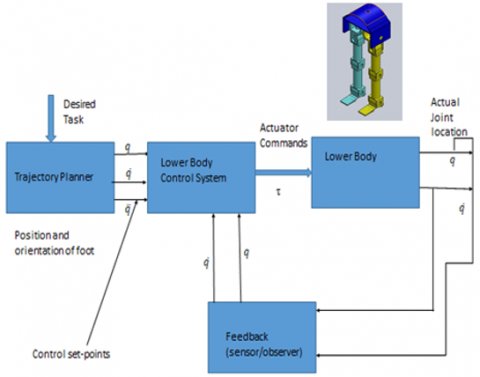
The control requires the knowledge of the mathematical model and some sort of intelligence. Whereas the required mathematical modelling is obtained from basic physical laws governing robot dynamics and associated devices [13]. A robot performs the specified tasks in its environment, which can be divided into two classes: Contact type tasks and non-contact type tasks. The non-contact type tasks involved manipulation of the end–effector in space to do desired work. While in contact-type tasks the end effector interacts with the environment. The foot of the lower body of the humanoid robot comes in contact with the ground and exerts a force on the ground. The ground force i.e. the combination of friction force and normal reaction force is applied to the body of the humanoid robot. The friction force is responsible to cause the motion in a forward direction and the body can move on the ground [14]. An individual joint of a manipulator is powered and driven by actuators that apply a force or a torque to cause the motion of the links. The actuator commands that move the manipulator and achieve the specified end effector motion, are provided by the manipulator control system [15]. These commands are based on the control set points generated from the set of joint torque time histories obtained by the trajectory planner [16]. The actual joint and/or end effector positions and their derivatives can be fed back to the control system to get accurate motion. The schematic diagram of a manipulator control system is shown in Figure 1. The dotted lines for the feedback indicate that the control system may employ feedback on the actual joint locations and velocities. The parameter $q$, $\dot{q}$ and $\ddot{q}$ and $\tau$ and so on.
Figure 1. Block diagram of lower body control system
The dynamic control of a manipulator's motions and /or interaction forces requires knowledge of forces or torque that must be exerted on the manipulator's joints to move the kinks and the end effector from the present location to the desired location, with or without the constraints of a particular planned end-effector trajectory, and or planned end –effector force/torque.
In both the situations of the desired end–effector location and the desired end effector force, the control of the individual joint’s location is important. Hence it is an obvious requirement that each joint is controlled by a position servo. If the lower body of the robot is to move very slowly or to move one joint at a time, then the control is simple because coupled dynamics forces are negligible.
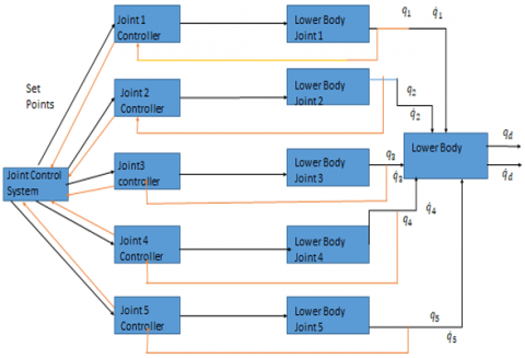
Each joint can be controlled independently by using a simple control system, which produces a joint actuator forces/torque proportional to the required change in the joint variable. This is the proportional control algorithm. If the motion is fast, which are must for effective robot applications, all joints must move simultaneously. In this situation, the coupled dynamics forces are significant, and it is known that dynamics are nonlinear and complex. Joints cannot move independently, and a complex control algorithm will be required. The typical robot control architecture for an n-Degree of freedom manipulator (DOF) consists of a master control system to control and synchronize n-joints [17]. This master control is responsible for sending “set point” information to command to each of the joint controllers. The n-joints controllers use the set point information to command the joint actuator to move the joint. The joint controller may employ feedback to the master controller. The schematic of a typical control architecture for a manipulator control system is illustrated in Figure 2.
Figure 2. Control architecture for 5-Dof manipulator
2.1 Manipulator control problem
The task to be performed by a manipulator may require either the execution of specific motions of the end effector in free space and/or the application of specific contact forces at the end effector if the end effector is constrained by the environment. For a given manipulator, many techniques can be used to control it to perform in the desired manner. The performance and range of application of a manipulator are significantly influenced by the control scheme followed, as well as the way it is implemented [18]. The mechanical design and configuration design also greatly influence the control technique utilized and the performance of the manipulator. Depending on the control law employed to compute the joint torques, the control system is classified as either linear or nonlinear [19]. The design of the linear controllers based on the approximate linear model of the manipulator will be examined.
The effects of time-varying inertia, interaction torques, and nonlinear torques, of the dynamics model are ignored to simplify the control system. Servo control strategies such as proportional derivatives (PD) are considered. Finally, the method of computed torque control, which is based on a nonlinear control law will be considered.
2.2 Effect of damping factor on the system
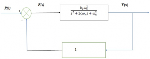
The control of a system consists of varying the inputs so that the closed loop dynamics of the systems have the desired properties; say the output $y$ follows the desired trajectory $y_d$. Feedback control explicitly uses the error signal, $\mathrm{e}=y-y_d$, the difference between the measured output $y$ and the desired output $y_d$, as a part of control law, to reduce the error and system sensitivity to the parameters in the dynamic model. The block diagram of this system with unity negative feedback is drawn in Figure 3.
Figure 3. Block diagram of a second-order linear system with unity feedback
If R(s)=Yd(s) is the Laplace transform of a set-point input, the closed-loop transfer function of the control system is
$\frac{Y(s)}{R(s)}=\frac{G(s)}{1+G(s)}=\frac{b_0 \omega_n^2}{s^2+2 \zeta \omega_n s+\left(1+b_0\right) \omega_n^2}$ (1)
The second-order linear characteristics equation of the closed-loop system is written in standard form as
$s^2+2 \xi \omega_n s+\omega_n^2=0$ (2)
where, ξ and ωn is the damping factor and natural frequency of the system.
The roots of the characteristics equation, r1, r2 which characterize the system’s time response to a given input, are
$r_1, r_2=-\xi \omega_n \pm \omega_n \sqrt{\xi^2-1}$ (3)
These roots determine the nature of time response of the system. If roots are real, then the response of the system is sluggish and non-oscillatory. If roots are complex conjugate, then the response of the system is oscillatory. The system response analysis helps in fixing the controller parameters that ensure closest possible trajectory tracking performance of a joint [20]. Depending on the values of the damping ratio, these roots can be real and unequal or real and equal or complex conjugate.
These three classes of the roots characterize the three types of time response of the systems. These three classes of roots arise with the value of damping ratio greater than unity, equal to unity and less than unity.
Case(i) Damping ratio greater than unity
A damping ratio greater than unity (ξ>1) gives the roots r1 and r2 as real and unequal. The roots r1 and r2 are
$r_1=-\xi \omega_n+\omega_n \sqrt{\xi^2-1}, r_2=-\xi \omega_n-\omega_n \sqrt{\xi^2-1}$
The time response is obtained by taking the inverse Laplace transform of the equation, which gives
$s^2+2 \xi \omega_n s+\omega_n^2=0$ (4)
$y(t)=1-\frac{e^{-\xi \omega_n \, t}}{2 \sqrt{\xi^2-1}}$$\left[\left(\sqrt{\xi^2-1}-\xi\right) e^{-\omega_n \sqrt{\left(\xi^2-1\right)} \, t}+\left(\sqrt{\xi^2-1}+\xi\right) e^{\omega_n \sqrt{\left(\xi^2-1\right)} \, t}\right]$ (5)
In this case, the system has sluggish and non-oscillatory behaviour and the system is overdamped.
Case(ii) Damping ration equal to unity
For a damping ratio equal to unity (ξ=1), both r1 and r2 are real and equal. The roots r1 and r2 are
$r_{1=}-\omega_n, r_{2=}-\omega_n$
and the time response of the system is
$y(t)=1-\left[1-e^{-\omega_n t}-\omega_n t e^{-\omega_n t}\right]$ (6)
Under this condition, the system exhibits the fastest possible non-oscillatory, overshoot-free response and it is critically damped.
Case(iii) Damping ratio less than unity
A damping ratio greater than unity (ξ<1) gives the roots r1 and r2 complex conjugates of each other.
The time response is obtained by taking the inverse Laplace transform of the equation, which gives
$y(t)=1-\frac{e^{-\xi \omega_n t}}{2 \sqrt{\xi^2-1}}$$\sin \left(\omega_n \sqrt{\left(1-\xi^2\right)} t+\tan ^{-1} \frac{\sqrt{\left(1-\xi^2\right)}}{\xi}\right)$ (7)
In this case, the system has an oscillatory behaviour and is underdamped.
From the above analysis, it is observed that the linear second order system is stable for all values of damping ratio, although the behaviour may be oscillatory or non-oscillatory.
A humanoid control system cannot allow an oscillatory response for obvious reasons. For instance, in a pick and place operation, an oscillating end effector may strike against the object before picking it to manipulate. Hence the highest possible speed of response and yet non oscillatory response dictates that the controller design parameters shall be chosen to have the damping ratio ξ=1 or at least close to it but less than unity.
2.3 Model of a manipulator joint
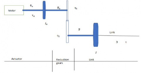
A common drive system for many industrial robots consists of an electric motor as the actuator and provide the torque to the joint. The schematic of an actuator gear link assembly of a rotary joint shown in Figure 4.
The gear ratio ‘η’ is defined as:
η = number of teeth on the gear of link shaft/number of teeth on the gear of actuator shaft. The gear ratio η is greater than 1 for a reduction gear. The gear ratio causes a reduction of the actuator speed $\dot{\theta}_a$ to $\dot{\theta}$, the speed of the link and increase of the actuator torque τa to τ, the torque applied to the link (the load) as given by
$\tau=\eta \tau_a$ (8)
$\dot{\theta}=\frac{1}{\eta} \dot{\theta}_a$ (9)
$\theta=\frac{1}{\eta} \theta_a$ (10)
where, Ɵa is the angular displacement of the actuator shaft and Ɵ is the joint angular displacement.
Figure 4. Actuator-gear-link mechanism
The link torque, when reflected to the actuator side, is scaled down by a factor η, the gear ratio. If Ia is the inertia of rotor of the actuator shaft and Ba is the viscous friction coefficient at the actuator bearings, for the rotational mass-damper system, the torque required at the actuator shaft is given by
$\tau_a=I_a \ddot{\theta}_a+B_a \dot{\theta}_a+\frac{\tau}{\eta}$ (11)
$\tau_a=I_a \ddot{\theta}_a+B_a \dot{\theta}_a+\frac{(I \ddot{\theta}+B \dot{\theta})}{\eta}$ (12)
where, I is the inertia of the load and B is the viscous friction coefficient for load. The Eq. (11) can be written in terms of the actuator shaft variable as.
$\tau_a=\left(I_a+\frac{I}{\eta^2}\right) \ddot{\theta}_a+\left(B_a+\frac{B}{\eta^2}\right) \dot{\theta}_a$ (13)
Or in terms of link variables as
$\tau=\left(I+\eta^2 I_a\right) \ddot{\theta}+\left(B+\eta^2 B_a\right) \dot{\theta}$ (14)
The nonlinearity term like viscous force, backlash, joint damping and air damping were discarded. The reason behind this, the system will work inside the closed room, hence there is no such effect disturb the system behavior.
The link torque τ is obtained from the dynamic model of the joint. The dynamic equation of the joint i is rewritten as below
$\tau=\sum_{j=1}^n M_{i j}(q) \ddot{q}_j+\sum_{\substack{j=1 \\ \text { for } i=1,2, \ldots, n}}^n \sum_{k=1}^n h_{i j k} \dot{q}_j \dot{q}_k+G_i$ (15)
In above equation, gravity loading G is significant in gravity environment only and comes into effect whenever motion is against gravity. The equation does not include the effect of friction, backlash, and elastic deformation. Backlash is difficult to model and elastic deformation and static friction are highly nonlinear and complex to model. The viscous friction is directly proportional to the velocity and can be included in the model. Hence the equation is modified as below to include the contribution of viscous friction.
$\tau=\sum_j M_j \ddot{\theta}_j+\sum_i \sum_k h_{j k} \dot{\theta}_j \dot{\theta}_k+B \dot{\theta}+G$ (16)
where, B is the viscous friction coefficient at the link bearings.
The term in equation is split into linear decoupled and nonlinear interacting terms.
The two linear decoupled terms are $M \ddot{\theta}$ from the first summation term for link i and the third term $B \dot{\theta}$. The remaining terms in equation are nonlinear interacting term and grouped together and denoted as ‘d’ i.e.
$d=\sum_{j \neq i, j=1}^n M_j \ddot{\theta}_j+\sum_j \sum_k h_{j k} \dot{\theta}_j \dot{\theta}_k+G$ (17)
Thus the equation can be written as
$\tau=M \ddot{\theta}+B \dot{\theta}+d$ (18)
Substituting τ from equation and rearranging, the actuator torque is obtained as
$\left(I_a+\frac{M}{\eta^2}\right) \ddot{\theta}_a+\left(B_a+\frac{B}{\eta^2}\right) \dot{\theta}_a+\frac{d}{\eta}$ (19)
In the case of highly geared manipulators (η≫1), it is quite reasonable to ignore the contribution of the nonlinear interacting terms d and still guarantee a good trajectory tracking performance by the controller.
Neglecting the nonlinear terms, the actuator torque reduces to the simple form
$\tau_a=\left(I_{\text {eff }}\right) \ddot{\theta}_a+\left(B_{\text {eff }}\right) \dot{\theta}_a$ (20)
where, Ieff is the effective inertia and Beff is the effective damping with
$I_{\text {eff }}=\left(I_a+\frac{M}{\eta^2}\right), B_{\text {eff }}=\left(B_a+\frac{B}{\eta^2}\right)$
Because the configuration dependent terms M is reduced by a factor η2, with η≫1), Ieff is almost constant for highly geared manipulators.
2.4 Model of a DC motor
The schematic diagram of an armature controlled permanent magnet DC motor is shown in Figure 5. Motors with field excitation provided by permanent magnets are preferred for robotics applications. Such motors are labelled permanent magnet DC motors.
Figure 5. Permanent magnet DC motor
With references to the schematic diagram, the control signal to the DC motor is applied at the armature terminals in the form of armature voltage ea. The motor torque $\tau_a$ is related to the armature current ia as
$\tau_a=K_T i_a$ (21)
where, KT is the motor torque constant. The armature current directly controls the torque generated by the actuator. The back emf $e_b$ induced in the armature winding is given by
$e_b=K_b \dot{\theta}_a$ (22)
where, Kb is the back emf constant. Applying the Kirchoff’s voltage law for the circuit of figure gives
$e_a=e_b+i_a R_a$ (23)
where, ea is the emf across armature and Ra is the armature resistance. Substituting eb from equation gives
$e_a=K_b \dot{\theta}_a+i_a R_a$ (24)
Thus, the armature voltage is adjusted, depending on the commands generated by the manipulator control system, which specify the torque required from the actuator. The continuous adjustment of the armature voltage ea is carried out by the motor driver circuitry so that the desired current $i_a$ flows through the armature windings. The schematic of a motor driver circuitry is shown in Figure 6.
2.5 Partitioned Proportional Derivative (PPD) control scheme
Since the system is nonlinear due to presence of second order derivative in the mathematical modelling. Linear PID control system would not capable to handle the nonlinear system. A nonlinear control theory were adopted for joint control system.
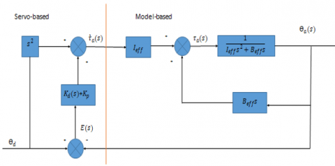
A linear controller based on a partitioned proportional derivative control strategy is slightly different from a simple PD controller. It is useful for systems that are more complex. The controller is partitioned into two parts; a model-based portion and a servo portion, such that the joint parameters (Ieff and Beff appear only in the model-based portion [21]. The approximate model of the manipulator joint developed in previous section is used to implement this controller. The block diagram of this controller is shown in Figure 7.
The portion to the right of the partitioned line is physical system, the model-based portion and to the left of the partitioned line is the servo based control system, usually implemented in a computer or microcontroller.
Figure 7. Partitioned PD controller for trajectory control
The model-based portion of the control law computes the command torque based on the system parameter Ieff and Beff. The Laplace of the approximate model of the joint is
$\tau_a(s)=\left(I_{e f f} s^2+B_{e f f} s\right) \theta_a(s)$ (25)
The model-based control law defines the actuator toque using a structure similar to that of equation, i.e.
$\tau_a(s)=I_{e f f} \hat{\tau}_a(s)+B_{e f f} s \theta_a(s)$ (26)
where, $\grave{\tau}_a(s)$ is the torque value specified by the servo portion to control a unit inertia.
From Eq. (24) and Eq. (25)
$\grave{\tau}_a(s)=s^2 \theta_a(s)$ (27)
This is the equation of motion for a system with unit inertia. Thus, the model based law effectively reduced the system to that of unit inertia system. In other words, the physical system appears to be a unit-inertia system to the servo portion [22].
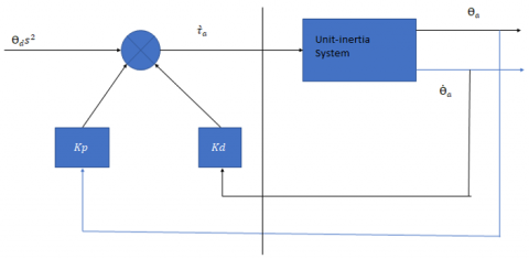
Figure 8. Simplified PPD controller for control of unit-inertia system
The servo portion of the controller is based on the error in actuator position and its derivative. These servo errors are computed as
$E(s)=\theta_d(s)-\theta_a(s)$ (28)
and $s E(s)=s \theta_d(s)-s \theta_a(s)$ (29)
where, Ɵd(s) is the desired joint displacement of the actuator shaft. The servo portion of the control law makes use of the feedback to modify the system behaviour. Because the model –based portion of the control law design becomes very simple. The controller is simply required to control a system of unit inertia with no friction and stiffness [16]. Assuming that the sensors are capable of detecting position and velocity, a proportional derivative control scheme can be used to control the system of mass /inertia. The control system using the PD control scheme with position and velocity feedback for the control of unit inertia is shown in Figure 8.
The control law for the servo portion is specified with two controller gain parameters, the proportional constant Kp, and the derivative constants Kd as
$\grave{\tau}_a(s)=s^2 \theta_d(s)+K_d s E(s)+K_p E(s)$ (30)
Combining Eqns. (28-30), the control law becomes
$s^2 \theta_a(s)=s^2 \theta_d(s)+K_d s E(s)+K_p E(s)$ (31)
The error dynamics of the PPD controller using equation, is given by
$s^2 E(s)+K_d s E(s)+K_0 E(s)=0$ (32)
Eq. (31) is identical to the characteristic equation of the second order linear system. Thus, the partitioned PD controller reduces the system to that of a linear second –order systems. Comparing equation with equation, gives the natural frequency of the system as;
$\omega_n=\sqrt{K_p}$ (33)
and the damping ratio as
$\xi=\frac{K_d}{2 \sqrt{K_p}}$ (34)
From equation, it is clear that any desired second –order performance of the control system is possible by the choice of proper control gains, Kp and Kd.
The controller for the manipulator should be critically damped, i.e., ξ=1.
Hence for critically damped performance
$K_d=2 \sqrt{K_p}=2 \omega_n$ (35)
2.6 Setting of gain parameter
The equation specifies the methodology for setting the methodology for setting the control gains Kp and Kd. A direct consequence of control law, equation, is that the servo error at any instant of time is zero provided there is no initial error and the computation time for the computer is zero, i.e., the actuator torque is computed as a continuous function of time.
In reality, the time taken to compute the servo error, the PD law control gains and to command a new value of torque, is nonzero and is known as the cycle time. This the resulting command torque $\grave{\tau}_a(s)$ is a staircase function and the servo error are non-zero at the beginning of each cycle.
The controller will reduce this nonzero servo error to zero during each cycle. Hence the actual trajectory tracked will be close to, but not exactly the same as desired trajectory. Apart from a damping ratio of unity, another factor that constraints the selection of control gains in the flexibility of links, which are assumed to be rigid bodies in the development of the joint model. The un-modelled structural flexibility of the link and other mechanical elements produces resonance at frequencies other than natural frequency. Because these structural flexibilities have been ignored, the controller must be designed so as not to excite these un-modelled resonances.
The lowest un-modelled resonance, which corresponds to the maximum value of the effective inertia seen by the actuator, Imax has a resonance frequency
$\omega_{\text {res }}=\omega_o \sqrt{\frac{I_0}{I_{\max }}}$ (36)
where, ωo is the structural frequency when the effective inertia is Io.
To prevent exciting these structural oscillations and also ensure structural stability, the controller natural frequency ωn must be limited to 0.5ωres, i.e.
$\omega_n \leq 0.5 \omega_{\text {res }}$ and $K_p \leq\left(0.5 \omega_o\right)^2 \frac{I_o}{I_{\max }}$ (37)
The natural frequency of individual link were obtained as follows
$\omega_n=\sqrt{\frac{3 E I}{L^3 M}}$ (38)
Based on these parameters the control gain Kp and Kd are computed.
Table 1 shows the approximate gain values for the different joint controller.
Table 1. Tuning parameter of the joint controller
|
Joint Controller(PD) |
Kp |
Kd |
|
Joint Controller1 |
65 |
32 |
|
Joint Controller2 |
68 |
30 |
|
Joint Controller3 |
72 |
34 |
|
Joint Controller4 |
65 |
38 |
|
Joint Controller5 |
70 |
34 |
Gain parameter of controller improves the stability of the system. Gain helps the controller to reach to the desired position.
Each joint of a manipulator was viewed as an individual system to be controlled for the simplified and linear controllers based on the PD and PID control scheme were examined for the simplified SISO model [20]. More realistic problem is the control of an n-DOF manipulator as a single system. A control scheme that makes direct use of the complete dynamics model of the manipulator to cancel the effect of gravity, Coriolis and centrifugal force, friction and the manipulators inertia tensor [23].
The dynamic model of the n-DOF manipulator based on the rigid body dynamics gives the nx1 vector of joint torques.
$\tau=M(q) \ddot{q}+H(q, \dot{q})+\dot{G}(q)$ (39)
where, M(q) is the nxn inertia matrix, $H(q, \dot{q})$ is the nx1 vector of centrifugal and Coriolis torques, G(q) is the nx1 vectors of gravity torques and the q(t), $q \dot{(} t)$ and $q \ddot{(} t)$ is the joint positions, velocities and accelerations respectively. Recall that q is the generalized joint variables.
Thus the Multi-Input –Multi output (MIMO), nonlinear dynamics model of n-DOF manipulator becomes
$\tau=M(q) \ddot{q}+H(q, \dot{q})+G(q)$ (40)
The design of a nonlinear control system based on the complicated model given by the equation, is considered now.
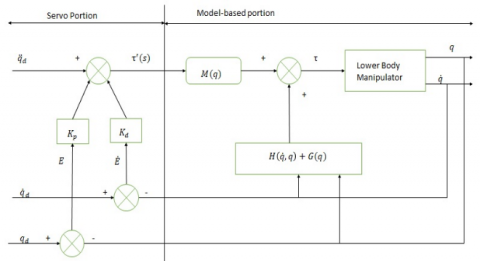
Because this controller is based on a more accurate dynamic model of manipulator, it provides better trajectory performances than linear controllers do. The controller discussed here employs the computed torque control law to modify the system effectively decouple and linearize it. The computed torque control scheme also comprises two portions- a model based and a servo portion. The model-based portion defines the nx1 vector of control torques τ using a structure.
$\tau=M(q) \grave{\tau}+H(q, \dot{q})+\dot{G}(q)$ (41)
where, $\grave{\tau}$ is the nx1 torque vector specified by the servo portion.
$\grave{\tau}=\ddot{q}$ (42)
Thus, the model based portion effectively linearizes as well as decouples the system dynamics by employing a nonlinear feedback of the actual positions and velocities of joints. The schematic representation of this nonlinear control scheme is shown in Figure 9.
Figure 9. Computed torque control law
The control law of the servo portion based on the nx1 vectors E and $\dot{E}$ of the servo errors in joint positions and velocities, respectively.
The servo portion of the computed torque control scheme is, therefore, defined as
$E(t)=q_d(t)-q(t)$ (43)
and $\left.E(t)=\dot{q}_d(t)-q \dot{(} t\right)$ (44)
where, q and qd denote the nx1 vectors of actual and desired joints positions respectively. The servo portion of the computed torque control scheme is therefore, defined as
$\ddot{q}=\ddot{q}_d +K_d{\dot{\dot{ \dot{E}+K_pE}}}$ (45)
where, Kp and Kd are the nxn matrices of position and velocity gains, respectively.
Usually, Kp and Kd are chosen as diagonal matrices with constant gains. This serves to decouple the error dynamics of the individual joints. The model of error behavior or error dynamics is obtained from
$\ddot{q}=\ddot{q}_d+K_d \dot{E}+\dot{\dot{\quad K_p}} E$ (46)
or with $\ddot{E}=\ddot{q}_d-\ddot{q}$ (47)
$\ddot{E}+K_d \dot{E}+\dot{K_p} E$ (48)
This shows that the error dynamics of a closed –loop system is specified by as second order linear error equation. This vector equation is decoupled if Kp and Kdare diagonal matrices with constant gain. Hence the error equation could be written on a joint by joint basis. For joint i the error equation is
$\ddot{e}_i+K_{d i} \dot{e}_i+K_{p i} e_i=0$ (49)
where, Kpiand Kdi are the position and velocity gains, respectively, for joint i.
For critically damped performance of joint, the relationship between Kpi and Kdi is obtained in equation i.e
$K_{d i}=2 \sqrt{K_{p i}}$ (50)
Observe that the computed torque controller employs nonlinear feedback to linearize dynamics and provides a better trajectory tracking performances than linear controllers, since it is based on a more accurate dynamics model, but the biggest limitation of this approach is that it is computationally more intensive and, hence highly expensive when compared to linear controllers.
Inaccuracies in the parameters of the manipulators in the dynamics model are other factors, which limit the manipulators performances.
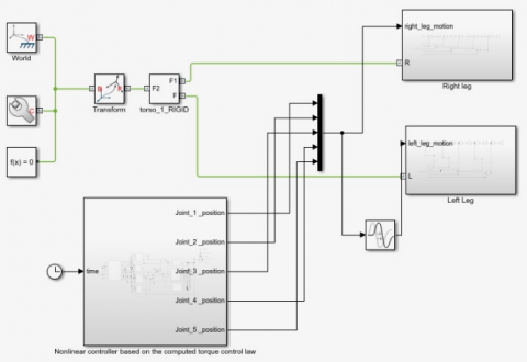
Figure 10. Simulink computed torque control
Figure 10 shows the schematic Simulink model of control system. The Coriolis and centripetal torque do not allow the link to reach the desired position of the robot. Computed torque control measures the inertia of the system and sense the signal to different motors controlling the humanoid feet to reach the desired position to reach to the desired position of humanoid feet to at actual position.
The input of the computed torque control is the input trajectory of joint. The nonlinear term of the CTC does not allow the link to reach the desired position. The CTC controller measure the error position and velocity of the joint. The PPD controller adjusted the torque and bring the joint into the desired position [24]. The Coriolis and the centripetal torque are nonlinear in nature. The CTC measured this variation and modifying the controller parameter based on the unit inertia system. The Simulink signal interacting with the physical system. So that one converter used for the interface. For this purpose, the SPS converter used to understand the interface the system. Figure 11 shows the interaction of the computed control to the lower body of the humanoid robot.
Figure 11. Interfacing of computed torque control to lower body of Humanoid
The interfacing of the CTC controller to the proposed model, the leg movement occurred for the plan trajectory and gait time has been noted. For a simple walk, the first, fourth and fifth joint trajectory has been implemented. During walk, the sequence of trajectory of hip joint, knee joint and ankle joint trajectory implemented, and movement of the leg observed for a gait period of 0.8 seconds [25]. A successful walk obtained. For the stable sudden turn, the first, second, fourth and fifth joint of the system comes into the action. During sudden turn, the second joint motion produced for the momentarily and it will stop. Afterward the same trajectory repeated as usual for the normal walk [1, 2].
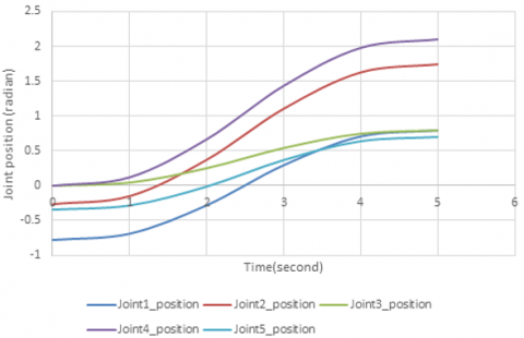
The simulation was carried out for the planned trajectory of the different joint. The fifth order polynomial equation has been used for the trajectory planning. The boundary condition applied at the starting and end of the trajectory. Initially the joint velocity and acceleration are zero. Hence there is no jerk coming at the start and the end of the motion. The fifth order polynomial equation creates the smooth trajectory of the joint movement. The simulation was carried out for the 5 second for the minimum and maximum values of the individual joints. Figure 12 shows the variation of desired joint position with respect to time.
The desired trajectory has smooth curve, so that during motion of the body parts, nominal jerk is coming on the joints. Joint1 started from the -0.7875 radian and reached to 0.7875radian of the target point.
Starting point of joint 2 is -0.2625 radians and reached to target point of 1.75 radians. The joint 3 started from the and reached to target point of 0.7875 radians. Similarly the joint 4 started from zero radians and reached to 2.1 radians and lastly the joint 5 started from -0.35 radians and reached 0.7 radians During this trajectory, the joints are touching the intermediate position.0.020501987 N-m to 0.04131821 N-m to a maximum value of 0.04131821 N-M.
Figure 12. Joint position with respect to time
Actual joint position
The simulation was carried out for the computed torque control law on the lower body of the Humanoid robot. The error between the desired joint position and the actual joint position evaluated for the planned trajectory of the individual joint.
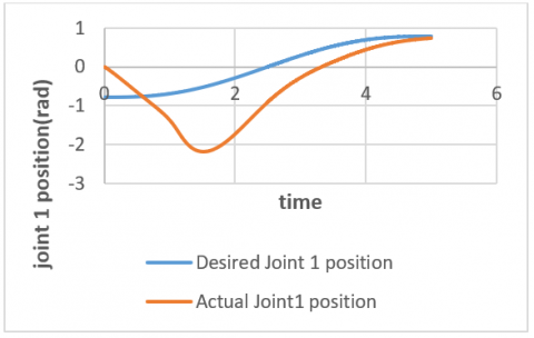
Figure 13. Comparison of joint 1 desired position to actual position
Figure 13 shows the desired joint position and actual joint position of joint 1. The starting desired point of joint 1 is -0.7875 radian but the actual joint starting point of joint 1 is 0 radian. At the time of t=0 seconds the joint 1 is starting from the -0.7875 radians, but the controller assumes the zero position of the actual joint1.Afterwards, the partitioned PD controller controls the joint position and reaching to the target point. During this movement there is overshoot of the actual joint position. This overshoot problem can be discarded by the assuming zero position of desired trajectory of joint 1. At the end of time t=5 seconds the actual joint position 0.7875 radians achieved by the joint 1 without any oscillation.
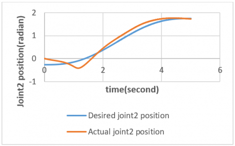
Figure 14. Comparison of joint 2 desired position to actual position
Figure14 shows the desired joint position and actual joint position of joint 2. The starting desired point of joint 2 is -0.2625 radian but the actual joint starting point of joint 2 is 0 radian.
At the time of t=0 seconds the joint 2 is starting from the -0.2625 radians, but the controller assumes the zero position of the actual joint2.Afterwards the partitioned PD controller controls the joint position and reaching to the target point. During this movement there is overshoot of the actual joint position. This overshoot problem can be discarded by the assuming zero position of desired trajectory of joint 1. At the end of time t=5 seconds the actual joint position 1.3 radians, that is not achieved by the joint 2. There is an error of 0.02 radians. This error can be discarded by the tuning of PD controller parameter.
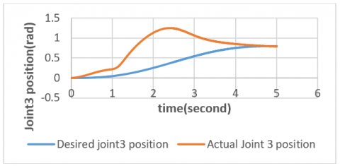
Figure15 shows the desired joint position and actual joint position of joint 3. The starting desired point of joint 2 is 0 radian and the actual joint starting point of joint 3 is 0 radian.
Figure 15. Comparison of joint 3 desired position to actual position
At the time of t=0 seconds the joint 3 is started from the zero radian and targeted to goal point of 0.7875 radians. The partitioned PD controller controls the joint position and reaching to the target point. During this movement there is overshoot of the actual joint position. At the end of time t=5 seconds the actual joint position 3 is 0.781 radians, which is slightly far away from the target desired position. There is an error of 0.006 radians. This error can be discarded by controlling the joint velocity of joint 3 by adjusting the velocity tuning parameter of PD controller. Figure 16 shows the desired joint position and actual joint position of joint 4. The starting desired point of joint 4 is 0 radian and the actual joint starting point of joint 4 is 0 radian.
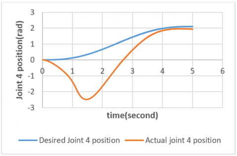
Figure 16. Comparison of joint 4 desired position to actual position
At the time of t=0 seconds the joint 4 is started from the zero radian and targeted to goal point of 2.1 radians. The partitioned PD controller controls the joint position and reaching to the target point.
During this movement there is overshoot of the actual joint position. At the end of time t=5 seconds the actual joint position 4 is 1.92 radians, which is slightly far away from the target desired position. There is an error of 0.18 radians. This error can be discarded by controlling the joint velocity of joint 4 by adjusting the tuning parameter of PD controller. During this movement of the joint, there is no oscillation in the movement. Figure 17 shows the desired joint position and actual joint position of joint 5. The starting desired point of joint 5 is -0.35 radian and the actual joint starting point of joint 5 is 0 radian.
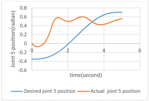
Figure 17. Comparison of joint 5 desired position to actual position
At the time of t=0 seconds the joint 4 is started from the -0.35 radian and targeted to goal point of 0.7 radians. The partitioned PD controller controls the joint position and reaching to the target point. During this movement there is overshoot of the actual joint position. At the end of time t=5 seconds the actual joint position 4 is 0.562 radians, which is slightly far away from the target desired position. There is an error of 0.138 radians. This error can be discarded by controlling the joint velocity of joint 5 by adjusting the tuning parameter of PD controller. During this movement of the joint, there is no oscillation in the movement.
A simple distributed master and slave control architecture adopted fir the joint movement control. The partitioned PD control law controls the nonlinear system very efficiently. The controller gain parameter was selected on the material stiffness and the natural frequency of the system. The system was designed for the critical damped, so that fast non-oscillatory behaviour of the joint is obtained. Some of the oscillation were observed due to discarding of the non-linearity term. This non-linearity can be removed from the system by increasing the controller gain vales. However, these values cannot go to a high values due to resonance occurs.
[1] Burghart, C., Mikut, R., Stiefelhagen, R., Asfour, T., Holzapfel, H., Steinhaus, P., Dillmann, R. (2005). A cognitive architecture for a humanoid robot: A first approach. In 5th IEEE-RAS International Conference on Humanoid Robots, pp. 357-362. https://doi.org/10.1109/ICHR.2005.1573593
[2] Kanda, T., Ishiguro, H., Imai, M., Ono, T., Mase, K. (2002). A constructive approach for developing interactive humanoid robots. In IEEE/RSJ International Conference on Intelligent Robots and Systems, 2: 1265-1270. https://doi.org/10.1109/IRDS.2002.1043918
[3] Rosenblatt, J.K., Payton, D. (1989). A fine-grained alternative to the subsumption architecture for mobile robot control. In Proceedings of the IEEE/INNS International Joint Conference on Neural Networks, 2: 317-324.
[4] Brooks, R. (1987). A hardware retargetable distributed layered architecture for mobile robot control. In Proceedings. 1987 IEEE International Conference on Robotics and Automation, 4: 106-110. https://doi.org/10.1109/ROBOT.1987.1088016
[5] Ly, D.N., Regenstein, K., Asfour, T., Dillmann, R. (2004). A modular and distributed embedded control architecture for humanoid robots. In 2004 IEEE/RSJ International Conference on Intelligent Robots and Systems (IROS) (IEEE Cat. No. 04CH37566), 3: 2775-2780. https://doi.org/10.1109/IROS.2004.1389829
[6] Wang, Y., Butner, S.T.E.V.E.N.E. (1987). A new architecture for robot control. In Proceedings. 1987 IEEE International Conference on Robotics and Automation, 4: 664-670. https://doi.org/10.1109/ROBOT.1987.1087952
[7] Kuroki, Y., Fujita, M., Ishida, T., Nagasaka, K.I., Yamaguchi, J.I. (2003). A small biped entertainment robot exploring attractive applications. In 2003 IEEE International Conference on Robotics and Automation (Cat. No. 03CH37422), 1: 471-476. https://doi.org/10.1109/ROBOT.2003.1241639
[8] Simmons, R., Apfelbaum, D. (1998). A task description language for robot control. In Proceedings. 1998 IEEE/RSJ International Conference on Intelligent Robots and Systems. Innovations in Theory, Practice and Applications (Cat. No. 98CH36190), 3: 1931-1937. https://doi.org/10.1109/IROS.1998.724883
[9] Khatib, O. (1987). A unified approach for motion and force control of robot manipulators: The operational space formulation. IEEE Journal on Robotics and Automation, 3(1): 43-53. https://doi.org/10.1109/JRA.1987.1087068
[10] Mansard, N., Stasse, O., Evrard, P., Kheddar, A. (2009). A versatile generalized inverted kinematics implementation for collaborative working humanoid robots: The stack of tasks. In 2009 International Conference on Advanced Robotics, pp. 1-6.
[11] Posadas, J.L., Poza, J.L., Simó, J.E., Benet, G., Blanes, F. (2008). Agent-based distributed architecture for mobile robot control. Engineering Applications of Artificial Intelligence, 21(6): 805-823. https://doi.org/10.1016/j.engappai.2007.07.008
[12] Erhart, S., Sieber, D., Hirche, S. (2013). An impedance-based control architecture for multi-robot cooperative dual-arm mobile manipulation. In 2013 IEEE/RSJ International Conference on Intelligent Robots and Systems, pp. 315-322. https://doi.org/10.1109/IROS.2013.6696370
[13] Feil-Seifer, D., Mataric, M.J. (2008). B 3 IA: A control architecture for autonomous robot-assisted behavior intervention for children with Autism Spectrum Disorders. In RO-MAN 2008-The 17th IEEE International Symposium on Robot and Human Interactive Communication, pp. 328-333. https://doi.org/10.1109/ROMAN.2008.4600687
[14] Galindo, C., Gonzalez, J., Fernandez-Madrigal, J.A. (2006). Control architecture for human–robot integration: application to a robotic wheelchair. IEEE Transactions on Systems, Man, and Cybernetics, Part B (Cybernetics), 36(5): 1053-1067. https://doi.org/10.1109/TSMCB.2006.874131
[15] Naumann, M., Wegener, K., Schraft, R.D. (2007). Control architecture for robot cells to enable plug'n'produce. In Proceedings 2007 IEEE International Conference on Robotics and Automation, pp. 287-292. https://doi.org/10.1109/ROBOT.2007.363801
[16] Khatib, O., Burdick, J. (1986). Motion and force control of robot manipulators. In Proceedings. 1986 IEEE International Conference on Robotics and Automation, 3: 1381-1386. https://doi.org/10.1109/ROBOT.1986.1087493
[17] Kuffner, J., Nishiwaki, K., Kagami, S., Inaba, M., Inoue, H. (2005). Motion planning for humanoid robots. In Robotics research. The Eleventh International Symposium, pp. 365-374. https://doi.org/10.1007/11008941_3
[18] Liu, H., Iberall, T., Bekey, G.A. (1989). Neural network architecture for robot hand control. IEEE Control Systems Magazine, 9(3): 38-43. https://doi.org/10.1109/37.24810
[19] Kim, J.Y., Park, I.W., Lee, J., Kim, M.S., Cho, B.K., Oh, J.H. (2005). System design and dynamic walking of humanoid robot KHR-2. In Proceedings of the 2005 IEEE International Conference on Robotics and Automation, pp. 1431-1436. https://doi.org/10.1109/ROBOT.2005.1570316
[20] Bharadwaj, D., Mishra, N., Pathak, M. (2022). Kinematic and singularity analysis of 10 DOF lower body of humanoid robot. Mathematical Modelling of Engineering Problems, 9(2): 484-490. https://doi.org/10.18280/mmep.090226
[21] Kanehiro, F., Fujiwara, K., Kajita, S., Yokoi, K., Kaneko, K., Hirukawa, H. (2002). Open architecture humanoid robotics platform. In Proceedings 2002 IEEE International Conference on Robotics and Automation (Cat. No. 02CH37292), 1: 24-30. https://doi.org/10.1109/ROBOT.2002.1013334
[22] Mayne, D. (1966). A second-order gradient method for determining optimal trajectories of non-linear discrete-time systems. International Journal of Control, 3(1): 85-95. https://doi.org/10.1080/00207176608921369
[23] Park, J.H., Kim, K.D. (1998). Biped robot walking using gravity-compensated inverted pendulum mode and computed torque control. In Proceedings. 1998 IEEE International Conference on Robotics and Automation (Cat. No. 98CH36146), 4: 3528-3533. https://doi.org/10.1109/ROBOT.1998.680985
[24] Rohmer, E., Singh, S.P.N., Freese, M.C. (2013). V-REP: A versatile and scalable robot simulation framework. In Proceedings of the International Conference on Intelligent Robots and Systems (IROS), Tokyo, Japan, pp. 1321-1326. https://doi.org/10.1109/IROS.2013.6696520
[25] Bharadwaj, D., Prateek, M., Sharma, R. (2019). Development of reinforcement control algorithm of lower body of autonomous humanoid robot. International Journal of Recent Technology and Engineering (IJRTE), 8(1): 915-919.