Implementation of Data Analytics for the Accuracy of Service Time Prediction Models

Currently, there are computer repair services available that cater to individual consumers and companies who need computer repair services. In a day, data from computer repair services can receive many units of computer damage. To repair the damage, it takes a completion time in accordance with the specified time.

When the repair is completed, an agreement on the length of the repair is made (Service Level Agreement) with the consumer so that there is no misunderstanding. Even though the agreement and completion time have been determined, sometimes there are obstacles in the repair process, such as complexity in analysis, inappropriate comparisons, and spare part stock that is not yet available in the warehouse.

Time of repair needs to be considered for accuracy so that no one is harmed between consumers and service providers of repair services, both morally and materially. Data analytic techniques are one of the effective ways to predict the timeliness of repairs by integrating heterogeneous data from various sources which are then drawn into a conclusion and made into a prediction for strategic decision making [1]. In data analytics, there is a data mining process. Data mining is a specific process to find scientific and observable knowledge, such as patterns, association relationships, changes, peculiarities of data and the structure of data in databases and information storage [2]. Meanwhile, Decision trees have an important role in producing science, business, and engineering in various fields, including classes on the use of data mining techniques that are easy to understand, easy to use and produce excellent decision results [3].

J48 decision tree method produces an effective level of accuracy for predicting diabetes mellitus diagnosis [4].

The level of accuracy using the J48 decision tree [5] can be seen from the results of the confusion matrix calculation resulting from the weka data mining application [6]. Where the data in the matrix is the result of the evaluation of the performance of the weka data mining application [7]. Based on the explanation of the above phenomena, problems can be identified, namely: (1). Determination of the repair time from the agreed one is not on time due to the complexity of the analysis, inappropriate comparisons and the unavailability of spare part stock in the warehouse. (2). The inaccuracy of repair time results in losses between consumers and computer repair service providers, both morally and materially. From the formulation of the problem above, it can be concluded as follows: (a) Problem Statement The timing of computer repairs is still low, so there is no time prediction for the completion of computer repairs. (b) Research Question. The research question that can be asked in this study is "How does the application of the J48 decision tree method determine the accuracy and predictive model of computer repair time correctly?". As for the aims and objectives of this research are as follows: 1). Meaning. The purpose of this research is to apply the J48 decision tree method to determine the accuracy of computer repair time. 2). Purpose. The aim of this research is to determine the level of accuracy of the J48 decision tree method in determining the accuracy of computer repair time.

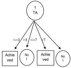
From the results in the table, it can be seen that the attribute with the highest gain is Turn Around Time (TAT), which is 0.79. Thus, Turn Around Time (TAT) can be a root node. Where, there are four attribute values of Turn Around Time (TAT), namely TAT less than equal to three (<=3), more than three (>3), less than equal to seven (<=7) and more than seven (>7). Of the four values, attribute values less than equal to three (<=3) and less than equal to seven (<=7) have classified cases into 1, namely the decision was achieved (achieved), and for attribute values more than three (>3) and more than seven (>7) have classified cases into 0, namely the decision was not achieved (not achieved) so that no further calculations are needed. From these results it can be described that the temporary decision tree looks like in Figure 1.

3.3 Implementation of J48 using weka 3.7.9

Data resolved and canceled cases (DATAR&C).csv processed using weka tools with the application of decision tree J48 which is the development of the C4.5 algorithm to determine the grouping of Service Level Agreement (SLA) achieved (achieved) or Service Level Agreement (SLA) not achieved (not achieved).

1) Pre-processing stages on weka 3.7.9

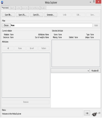
In the first stage weka is a pre-process, namely by entering the data resolved and canceled cases (DATAR&C).csv as the main dataset to be classified. The total dataset resolved&cancelled cases consisted of 5310 records and 4 attributes. Weka will explore the characteristics of the attributes of the dataset. The pre-process stages in Weka 3.7.9 can be seen in Figure 2 and Figure 3.

1.png

Figure 1. Decision tree calculation results node

2.png

Figure 2. Display of weka pre-process 3.7.9 before entering data

3.png

Figure 3. Display of weka pre-process 3.7.9 after entering data

The dataset resolved and canceled cases were processed using the J48 classifier technique with the output of a Service Level Agreement (SLA). The type of test used is cross validation [12]. The display of the classify panel on weka can be seen in Figure 4.

4.png

Figure 4. Panel classifier information

1. Choose: Selection of the classification algorithm to be used.

2. Use Training Set: Using training data sets.

3. Supplied test set: Using data testing.

4. Cross-validation: Data sharing.

5. Percentage Split: Percentage of splits or ramifications.

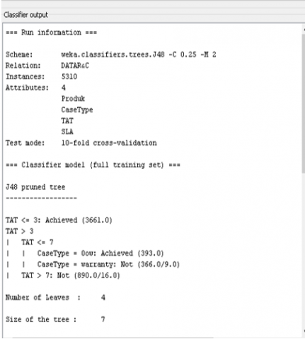
After doing the classifier technique from the dataset, and selecting the type of test used and then clicking start, the classifier output results come out. As in Figure 5.

5.png

Figure 5. Classifier output

The classification process [13] is influenced by the selected attributes that support to determine the service level group / Service Level Agreement (SLA) is achieved (achieved) and the Service Level Agreement (SLA) is not achieved (not achieved) based on the status of the product type (casetype).

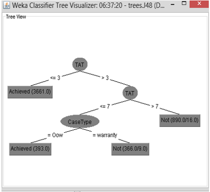
From the results of processing and testing using J48 on the dataset, the information is compiled in the form of a tree as shown in Figure 6.

6.png

Figure 6. J48 classification model in tree form

From the figure, it can be seen that Turn Around Time (TAT) is the root of the tree. If the Turn Around Time (TAT) can be completed in less than three days (<=3) warranty status, the classification results show achieved which means the product unit is repaired in accordance with the agreement on the length of repair with the customer. If the Turn Around Time (TAT) is more than three days (>3) warranty status, the product unit is repaired beyond the agreed length of repair, which means that the Service Level Agreement (SLA) was not achieved (not achieved). This does not apply if the Turn Around Time (TAT) is more than three days but less than equal to seven days (<=7) out of warranty (oow) status, then the repaired product unit is achieved. And if the product unit that is repaired, Turn Around Time (TAT) is more than seven days (>7) the status is out of warranty, then the agreement on the service level is not achieved (not achieved).

2) Evaluation using K-Fold Cross Validation

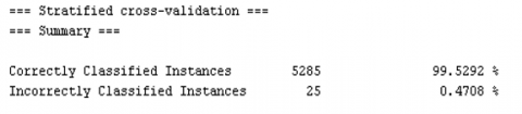
The results of the evaluation resulted in data that were classified correctly (Correctly Classified Instances) in accordance with the grouping of Service Level Agreement (SLA) achieved (achieved) and Service Level Agreement (SLA) not achieved (not achieved) by the algorithm as much as 99.5292% or as many as 5285 data and data that is classified but does not match the predicted class (Incorrectly Classified Instances) which should be in the Service Level Agreement (SLA) group was not achieved (not achieved) but was included in the Service Level Agreement (SLA) group achieved (achieved), which was 0, 4708% or as much as 25 data, as shown in Figure 7. Next is the calculation of the accuracy details.

7.png

Figure 7. Evaluation results using k-cross validation

True Positive (TP) Rate is data that has been classified as class "x" among all data that actually belongs to class "x". This is equivalent to remembering. In the Confusion Matrix, the diagonal elements are divided by the number of relevant lines, namely 4054 / (4054+25) = 0.99 SLA class achieved (achieved) and 1231 / (0+1231) = 1 for SLA class not achieved (not achieved). False Positive (FP) is the proportion of data that has been classified as class “x”, but belongs to a different class than previously predicted. In the confusion matrix, the number of column "x" classes under the diagonal element is divided by the number of rows from all other classes, namely 0 / 1231 = 0 for class SLA achieved (achieved) and 25 / 4079 = 0.006 class SLA is not achieved (not achieved).

Precision [14] or accuracy is ability to not display inappropriate documents with the needs of the user. In the matrix, the diagonal elements are divided by the number of relevant columns, namely 4054 / (4054 + 0) = 1 for the SLA class achieved (achieved) and 1231 / (1231+25) = 0, 980 for the SLA class not achieved (not achieved) . The calculation results from the accuracy details can be seen in Figure 8.

8.png

Figure 8. Class accuracy details

3.4 Analysis of results

The next process will calculate the average percentage of accuracy and error rate in the confusion matrix. The accuracy of the model is calculated using the confusion matrix [15]. Letters a and b in the table respectively indicate the SLA class was achieved (achieved) and the SLA was not achieved (not achieved).

This processing uses 5,310 records of data. Based on the results contained in the confusion matrix, the column represents a prediction, and the row represents the actual class. It can be seen that the number of correct predictions is (aa, bb) and the total number of incorrect predictions is (ab, ba). From the confusion matrix, it can be seen that 4,054 records in class aa are predicted to be correct as class a and as many as 25 records are predicted to be incorrect as the data group class SLA is achieved (achieved), because the record is predicted as class SLA is no bt achieved (not achieved). Furthermore, all records in class bb as many as 1,231 are predicted to be right as class SLA is not achieved (not achieved), from this result can be calculated the average percentage of success accuracy and error rate in the confusion matrix [16, 17].

Accuracy $=\frac{\text { the number of correct predictions }}{\text { total number of predictions }}=\frac{f_{11}+f_{00}}{f_{11}+f_{10}+f_{01}+f_{00}}$

Accuracy $=\frac{4054+1231}{4054+25+0+1231} \times 100 \%=99,5 \%$

$\text { Error rate }= \frac{\text { many wrong predictions }}{\text { total number of predictions }} =\frac{f_{10}+f_{01}}{f_{11}+f_{10}+f_{01}+f_{00}}$

Error rate $=\frac{25+0}{4054+25+0+1231} \times 100 \%=0,5 \%$

It can be concluded that the calculation of the percentage level of accuracy in the confusion matrix reaches a percentage value of 99.5% with an error rate or error rate of 0.5%, so that the dataset resolved and canceled cases are declared accurate using the J48 classifier method in determining time accuracy.