Block-Based K-Medoids Partitioning Method with Standardized Data to Improve Clustering Accuracy

There are two great statistics and computer science lessons: classification or supervised learning and clustering or unsupervised learning [1]. The emphasis of classification is on deriving a rule to assign new objects into a class [1-3]. Meanwhile, the principle of clustering is done based on similarities or distances (dissimilarities) [1, 2]. The inputs required in clustering are a measure of similarity or data that can be calculated for proximity. The k-medoids algorithm is one of the most well-known clustering methods. This method is more robust to noises or outliers than the k-means clustering [4]. One critical problem in the k-medoids algorithm is determining the initial medoids [5-7]. Simple and fast k-medoids (SFKM) and simple k-medoid (SKM) as medoid-based algorithms have been proposed [5, 7]. Both algorithms use a distance matrix to select the initial medoids with a specific formula. When medoids are non-unique objects, the SFKM algorithm suffers from possible empty clusters, and in the SKM algorithm, similar things may be in different groups. The first phase of the flexible k-medoids (FKM) ensures that no initial groups are empty and the medoids of identical objects are in the same groups [8]. Another issue in k-medoids clustering is the unpredictable number of iterations. The complexity of k-medoids clustering or Partitioning Around Medoid (PAM) is quadratic time, namely, $O\left(k(n-k)^2\right)$ [4, 5]. For this reason, some investigations have been conducted to reduce running time in k-medoids clustering [5, 9-11]. Reference [9] modifies the PAM algorithm that achieves an O(k)-fold speedup in the second phase of the algorithm by eagerly performing additional swaps in each iteration. The SFKM algorithm uses one initialization, namely objects in the initial group to update the medoid [5]. In contrast, the SKM method suggests twenty times initialization [7]. Like the SKM, the FKM algorithm randomly implements five to fifteen times to update the medoid based on the initial group members [8]. The purity algorithm uses the Davies-Bouldin Index to analyze groups to reduce the number of iterations in k-medoids [10], making this method suitable for numerical data. Hybridization of k-medoids with the crow search algorithm's characteristics (KMCSA) has been developed to eliminate the computational burden of the k-medoids algorithm. The KMCSA algorithm is claimed to be able to improve the balance between the exploration and exploitation processes of the k-medoids algorithm [11]. On the other hand, several real datasets in cluster analysis have mixed variables between categorical and numerical data. To overcome these data, one of which can standardize to adjust the size of variables (magnitude) and relative weight [12].  

The proximity (similarities or distances) between objects is calculated based on the data type. There are four data types in cluster analysis: nominal, ordinal, interval and ratio scale [4]. The basic rules in the measurement theory are the data results of the measurement on the stronger scale can be transformed into numbers on the weaker scale. The transformation from a lower to a larger scale is not permitted [4]. A general guideline in statistics is that the function for measuring lower data can be used for data on a larger scale. In some multivariate statistical methods, including cluster analysis, it is often useful when the measurement scales of all variables are either the same or at least similar. The allowed transformations on numerical data are linear transformations with a standardization formula as follows [12],

$z_{i j}=b x_{i j}+a(b>0)$          (1)

where, $x_{i j}\left(z_{i j}\right)$ denotes the value (standardized value) of the $j$ -th variable for $i$ -th object. The value that is often used is $b=\frac{1}{\sigma}$ and $a=-\frac{\mu}{\sigma}$, so that Eq. (1) can be rewritten as follows:

$Z_{i j}=\frac{x_{i j}-\mu}{\sigma}$          (2)

The transformation for the ratio scale also uses the value of $b=\frac{1}{x_{0 j}}$ and $a=0$, where $x_{0 j}$ denotes normalizing value, depending on cases that are met, for example, range, the maximum value of a variable, standard deviation, or mean. Meanwhile, the rank-based transformation is used for ordinal data [13].

In this research, we propose new method to reduce the number of iterations in the k-medoids algorithm. We use artificial data and eight real datasets from the University of California, Irvine (UCI) repository to evaluate the proposed method. This study also aims to examine the effectiveness of data standardization in increasing clustering accuracy. At the same time, we apply five of eight real datasets to compare the clustering accuracy between non-standardized data and several standardization methods. We implemented the partitioning methods (including the proposed method) and hierarchical clustering to achieve the second goal.

3.1 Hierarchical method

There are two general clustering methods: the hierarchical (agglomerative) method and the partition method. The steps in the agglomerative clustering for n objects are as follows [2],

(i) Start with n clusters, each containing a single entity and an n x n symmetric matrix of distances.

(ii) Search the distance matrix for the nearest pair of clusters. Let the distance between "most similar" clusters U and V be $d_{U V}$ .

(iii) Merge clusters U and V. Label the newly formed group (UV) and update the distance matrix.

(iv) Repeat steps (ii) and (iii) a total of (n-1) times.

In this paper, for step (iii), the distances between (UV) and other clusters W used average linkage, centroid linkage, complete linkage, weighted average linkage (McQuitty), and Ward's method [2].

3.2 Partitioning method (proposed)

For the partitioning method, we use k-means [20], simple and fast k-medoids [5], and modification of flexible k-medoids (proposed method). Reference [8] shows that a representative object of the block of the combined standard deviation and the sum of variable values as the initial medoids guarantees no empty initial groups.

In this paper, we modify the second stage of the flexible k-medoids. We adopted ideas from the second and third phases of SFKM to develop it. As the flexible k-medoids, the newly proposed method uses an object representative of the block of the standard deviation and the sum of variable values as initial medoids. We call the new way a block based k-medoids (Block-KM). To construct the Block-KM method, we define some parameters.

Suppose we have n objects with p-variables of numerical or categorical or mixed, then the standard deviation for an object $i$ with $p$-variables is as follows [8]:

$u_i=\sqrt{\frac{\sum_{l=1}^p\left(x_{i l}-\bar{x}_i\right)^2}{p-1}}$          (9)

where, $\bar{x}_i=w_i / p$; with $w_i$ is sum up of p-variables values as follows,

$w_i=\sum_{l=1}^p x_{i l}$          (10)

where, i=1, 2, ⋯, n; l=1, 2, ⋯, p. These parameters are used as a guide for selecting the initial medoids.

The average distance within cluster g-th, which has $n_g$ members for an object i-th, $\bar{D}_i$ defined as follows:

$\bar{D}_i=\frac{1}{n_g} \sum_{j=1}^{n_g} d_{i j}$          (11)

The total distance from all objects to their medoids, TD(k), is defined as follows,

$T D(k)=\sum_{g=1}^k \sum_{i=1}^{n_g} \sum_{l=1}^p\left|x_{g i l}-m_{g l}\right|$          (12)

where, $x_{g i l}$ is object i-th for variable l-th in the cluster g-th; and $m_{g l}$ is medoid cluster g-th for variable l-th. 

1.png

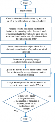
Figure 1. Flowchart of block k-medoids

Based on Eq. (9) to Eq. (12), then the flowchart of the Block-KM algorithm such in Figure 1. The detail of the algorithm is as follows,

Stage 1: Selection of the initial medoid

1-1 For each object, $i$ (i=1, 2, ⋯,n) calculated two parameters, Eq. (9) and Eq. (10).

1-2 Arrange all objects, first based on Eq. (9), $u_i$ in ascending order, then each block of the same standard deviation (if any), objects are sorted based on Eq. (10), $w_i$, also in ascending order.

1-3 For the first $k$ blocks of the combination of $u_i$ and $w_i$  (or may only block of $u_i$ ); select the first object from each block as the initial medoid.

1-4 Determine the members of k initial groups based on the distance of an object to the nearest medoid.

Stage 2: Finding the partitioned dataset

2-1 Update the current medoid in each cluster based on the object that minimizes the average distance to other things in its group. 

2-2 Obtain the cluster by assigning each object to the nearest medoid and calculate TD(k).

2-3 Repeat steps 2-1 and 2-2 until the TD(k) is equal to the previous one or a pre-determined number of iterations is attained, or the set of medoids does not change.

The novelty of Block-KM is the step for finding the partitioned dataset in the second stage. This process is easy because it uses one combination of initial medoids from the first stage (one initialization). The first phase of Block-KM is similar to the FKM (an illustrative example of the first stage [8]). The first phase of the Block-KM method indirectly grouped the data, especially when the data set consists of many identical objects or blocks of the same variance with the different sum of the values of the p-variables. In addition, in Block-KM, we always use the first object from the first $k$ block of a combination of deviation and sum on p-variables.

In comparison, the FKM or SKM algorithms randomly select the representative object as medoids. The Block-KM reduce the number of initialization from five (or more) to one time to obtain initial medoids. This step can reduce the number of iterations to achieve stability of total deviation.

3.3 Evaluation Indexes

We use clustering accuracy and adjusted Rand index to determine whether the two cluster results are similar. The clustering accuracy is defined as follows [21]:

$A c c=\frac{1}{n} \sum_{g=1}^k a_g$          (13)

where, n is the number of objects; k is the number of clusters; and $a_g$ is the number of objects in considered groups correctly assigned to the actual clusters. The range value of clustering accuracy is 0 (zero) to 1 (one). The larger this value, the better the accuracy.

Suppose that C is a clustering result under consideration and P is the true partition [22], then formulated the Adjusted Rand Index (ARI) as follows:

$A R I=\frac{2(a d-b c)}{(a+b)(b+d)+(a+c)(c+d)}$          (14)

where, a is the number of pairs of the objects placed in the same cluster in P and in the same group in C; b is the number of pairs in the same class in P but not in the same cluster in C, $c$ is the number of pairs in the same group in C but not in the same cluster in P, and d is the number of pairs in different groups in C and different classes in P. As with the clustering accuracy, the larger the ARI, the better the clustering results. We also apply the Purity and F-measure to evaluate the quality of the proposed method, especially for real datasets [23]. Both parameters have the same range and meaning with accuracy.

5.1 Experiment results of real data set

In this subsection, we discuss the algorithm precision of block k-medoids (proposed method) in terms of clustering accuracy. We also analyze the efficiency of Block-KM based on the required number of iterations to obtain the stability of total deviation. We have tried several transform methods and distance measures. However, we only describe the way that produces maximum clustering accuracy.

We applied the Manhattan, Euclidean and Canberra for iris and wine datasets. The maximum clustering accuracy of iris data was 95.3% for Canberra. This accuracy obtained via transformation by Eq. (1) with the value of $b=\frac{1}{s_j}$ (where $S_j$ is standard deviation) and a=0 for iris data. Meanwhile, the maximum clustering accuracy for wine and breast cancer datasets was 95.5% and 93.5% for Euclidean distance. We transform via Eq. (3) for wine data and Eq. (4) for breast cancer data before calculating the Euclidean distance.

We implement simple matching for all binary variables of vote data. The clustering accuracy of vote data is 86.6%. Then, we operate simple matching for 32 features of soybean small data. While; three of the 35 variables have an ordinal type tendency, so we transform by Eq. (3) before operating Eq. (6) and Eq. (8). With these terms, the clustering accuracy achieves a hundred percent for soybean small data.

For mixed datasets, we always use simple matching for categorical data. At the same time, we apply Manhattan or Euclidean distance for numerical data. Then, we use it to construct Eq. (8). The maximum accuracy of HD case 2 data was 82.8% via Manhattan distance for numerical data. We calculate the Euclidean distance for five numerical variables to get maximum accuracy of 82.8% in credit approval data. The maximum accuracy was 91.1% for zoo data. We transform one numerical variable in zoo data by Eq. (4) before executing Manhattan distance. We also implement the flexible k-medoids for eight real data sets with the same terms.

The comparison of precision algorithms based on the clustering accuracy for eight real datasets; is shown in Table 2. This comparison may be unfair because the method and distance used may differ. However, for the same purposes, namely, to get a good clustering, we tried to validate our proposed method based on the level of accuracy. The accuracy values for seven datasets by block k-medoids are generally comparable with other methods.

Table 2. The clustering accuracy of eight real datasets

Data Set	Block-KM	Other methods
1. Iris 2. Wine 3. Breast cancer 4. Vote 5. Soybean small 6. HD case 2 7. Credit approval 8. Zoo	95.3 95.5 93.5 86.6 100.0 82.8 82.8 91.1	92.0(a), 95.3(b), 97.3(c), 82.1(d) 92.7(b), 95.5(c) 93.5(c) 87.8(b), 93.1(c) 100(b,c,e), 98.9(d), 95.8(f) 84.2(c), 81.2(d), 81.0(g), 82.7(b), 82.8(c), 79.6(d), 81.2(g) 82.2(b), 96.0(c), 88.8(d), 89.9(g)

(a) Ref. [5], (b) Ref. [7], (c) Ref. [8], (d) Ref. [25], (e) Ref. [26], (f) Ref. [27], (g) Ref. [28]

Table 3. The adjusted Rand index, Purity, and F-measure for real datasets

Data Set	ARI	Purity	F-measure
1. Iris 2. Wine 3. Breast cancer 4. Vote 5. Soybean small 6. HD case 2 7. Credit approval 8. Zoo	0.868 0.863 0.760 0.535 1.000 0.429 0.431 0.922	0.953 0.955 0.972 0.866 1.000 0.828 0.828 0.921	0.953 0.955 0.972 0.866 1.000 0.828 0.828 0.639

To balance the evaluation of our proposed method, we calculate the adjusted Rand index, Purity and F-measure for eight real datasets. According to Table 3, the block k-medoids method produces high a Purity value for all real data sets. Then F-measure for iris, wine, breast cancer and soybean data is also high. Meanwhile, the F-measure value is less reliable for vote data with binary type and three real data sets with mixed-types, i.e., heart disease case 2, credit approval and zoo data. Furthermore, the adjusted Rand index is also high except for HD case 2 data, and credit approval data are not satisfied. Both datasets have mixed types with high variation.

In addition, we implement the number of ten iterations for steps 2-3 in the second phase. Figure 2 shows the plot between the number of iterations and the total deviation within a group, TD(k), divided by TD(k) of the first iteration (based on initial groups). According to Figure 2, the total distance of vote, heart disease case 2, and credit approval data achieve stability on the second iteration. These datasets required two iterations to obtain the total deviation within the group, not changes. The total distance does not change on wine and zoo data on the second and next iterations. Breast cancer data needed four iterations to get the stability of the total distance. Meanwhile, the total distance of the iris and soybean small data in the fourth iteration was equal to the fifth and subsequent iterations.

2.png

Figure 2. The plot of the total deviation weighted for each iteration of eight real datasets

The maximum number of iterations is five times for eight real datasets. Thus, a block k-medoids partitioning method is shorter than the original flexible k-medoids and simple k-medoids. The flexible k-medoids and simple k-medoids needed more than five times for initialization. Suppose the quality of the initial medoids of both algorithms is good. In that case, the number of iterations for each initialization may be similar to Block-KM, i.e., one to five iterations to obtain the stability of total deviation.

5.2 Experiment results of artificial data set

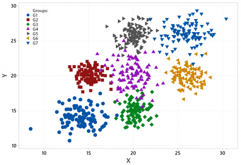
This subsection demonstrates the average adjusted Rand index and the number of iterations for artificial data. Although the number of iterations has no direct effect on clustering accuracy, it will impact on the steps required to obtain the final group. We constructed three various artificial data sets and executed hundred times. At the same time, we use the Euclidean method for numerical data and simple matching for categorical artificial data. We apply ten iterations for steps 2-3 in the second phase of Block-KM. Figure 3 shows an example of artificial data set for seven groups with two numerical data.

According to Table 4, the average adjusted Rand index for the three experiments was relatively high, with a standard deviation of less than 0.1.

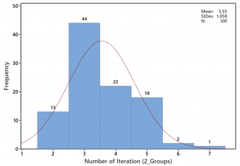
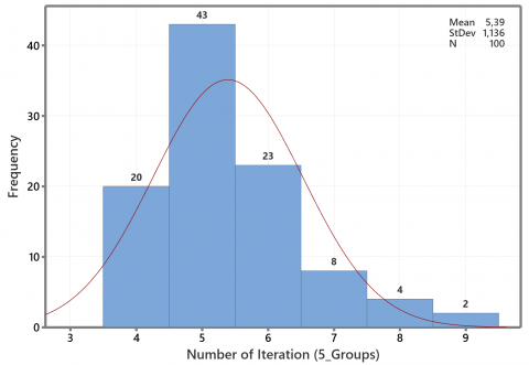
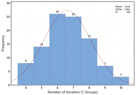
Based on one initialization of the first phase of the proposed method, the iteration profile is required to obtain the stability of the total deviation in the group, as shown in Figures 4 to 6. According to Figure 4, the majority iteration required for the stability of the total deviation is three iterations. Then, the highest iteration frequency for the five groups was five iterations, such as in Figure 5. Meanwhile, Figure 6 shows the range of iteration is four to ten, with a majority between six and seven iterations for seven groups. Although all three experiments show the number of iterations below ten, we do not claim that a new method always requires less than ten iterations. The quality of initial medoids and variation of the data set may cause the high required iteration number.

3.png

Figure 3. An example of artificial data set for seven groups

The iteration needed to get the final group from the proposed method is only done based on the initialization results in stage one. In contrast, flexible k-medoids and simple k-medoids require more than five initialization processes. For each initialization result, a number of iterations will be performed to get the final group. This means that if it is initialized $S$ times, and each takes $B$ iterations to get the final medoid, then the method takes (s.B) times to process. In comparison, the proposed method requires only $B$ times.

4.png

Figure 4. Profile of the iteration number for two groups of artificial data

5.png

Figure 5. Profile of the iteration number for five groups of artificial data

6.png

Figure 6. Profile of the iteration number for seven groups of artificial data

In addition, the block k-medoids also generate the same final group members. Whereas the flexible k-medoids and the simple k-medoids, as random-based methods, can produce different final group members. The last group of both methods rely on random outcomes. Therefore, we conclude that the block k-medoids method is more straightforward than flexible k-medoids or simple k-medoids. In addition, the ARI from the proposed method is also relatively high.

5.3 The comparison of clustering accuracy

This section describes the effectiveness of some ways to standardize data to increase the grouping accuracy. Then, the transformation method uses Eq. (2), Eq. (3), and Eq. (4) for ordinal and numerical data. We use five datasets: wine, breast cancer, HD case 2, credit approval and zoo data. For all datasets, we apply Euclidean distance for numerical data and simple matching for categorical data.

The wine and breast cancer data used hierarchical clustering with the linkage of average, centroid, complete, McQuitty, and Ward. In addition, we also apply the non-hierarchical method of k-means, simple and fast k-medoids, and block k-medoids. Grouping of soybean small, HD case 2, credit approval and zoo data used the same transformation technique and clustering method (except k-means). The k-means clustering was not applied because it was unsuitable for mixed data.

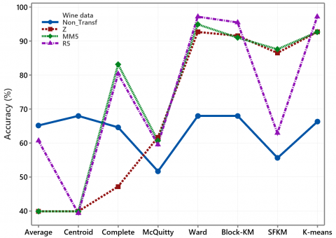
Wine data has a high variation; five of the thirteen variables contain outliers. For this data, we apply Eq. (3) and Eq. (4) by taking a value of f=5 with notation R5 (Rank use f=5) and MM5 (Min-Max use f=5). Figure 7 shows clustering accuracy for wine data on several transformations.

7.png

Figure 7. The plot of clustering accuracy for wine data

8.png

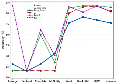
Figure 8. The plot of clustering accuracy for breast cancer data

Applying the hierarchical method with average and centroid linkage yields high accuracy for non-standardized data. All transformation methods improve clustering accuracy, especially with McQuitty, Ward, k-means, SFKM and Block-KM. Standardization based on Eq. (2) has not increased the accuracy with complete linkage.

As for the wine data, the thirty breast cancer variables have a high variation between zero and 4254. Applying k-means, SFKM, Block-KM, and Ward method on standardized breast cancer data effectively improve the accuracy. For this data, the transformation using Eq. (3) with a value of f=5 increases the accuracy for all hierarchical methods except the McQuitty method, as shown in Figure 8.

Three of eight HD case 2 variables are binary type, while five features have more than two categories. The five numerical variables of the HD case 2 data have a high variation. Implementing the hierarchical method with average and complete linkage, Ward, and Block-KM on standardized HD case 2 data effectively improves accuracy, as shown in Figure 9. The SFKM method is unsuitable for transformation using Eq. (3) because the two smallest objects are identical, so cause the number of groups formed is only one. In other words, the SFKM produces an empty group. The Block-KM can handle well for this case, as in Figure 9.

9.png

Figure 9. The plot of clustering accuracy for HD data

10.png

Figure 10. The plot of clustering accuracy for credit data

The credit approval data is exciting because it has mixed variables with binary, multinomial and continuous types. The hierarchical method with the linkage of average, centroid and McQuitty yielded the same accuracy for standardized and non-standardized data. Standardization in two new ways for six numerical data significantly improves clustering accuracy, especially with complete linkage, Block-KM and SFKM, as shown in Figure 10.

11.png

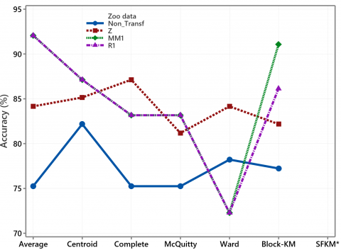
Figure 11. The plot of clustering accuracy for zoo data

As mentioned in sub-section 3.2, the flexible k-medoids and Block-KM are designed to solve the empty groups in the SFKM method. In the data zoo, there are several identical object blocks, which causes the SFKM method to not group the data into seven classes, either on the data without or with three transformations. Except for Ward's method, all transformation methods effectively increase clustering accuracy, as shown in Figure 11. We apply Eq. (3) and Eq. (4) to one numerical variable by taking the transformation multiplier of one because the other fifteen variables are binary.

According to Figure 7 to Figure 11, it can be seen that the standardized data can increase the accuracy of several clustering methods. This method is mainly for cluster analysis which is based on the partitioning method namely the k-means algorithm, the simple and fast k-medoids algorithm, and the newly proposed method. Hierarchical clustering using Ward's method improves accuracy, especially for wine, breast cancer, and HD case 2 data. For mixed data, i.e., zoo, HD case 2 and credit approval data, applying a hierarchical procedure with average linkage, centroid linkage, complete linkage and the McQuitty method also improves accuracy. Therefore, data standardization is an option for the five data sets in the hierarchical approach.   

5.4 The comparison of the average clustering accuracy on several methods and datasets

This subsection analyses the average clustering accuracy for all methods on each data set. We also discuss each technique's average clustering accuracy of all data sets.

12.png

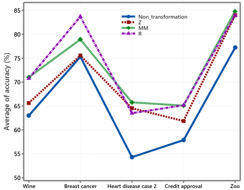
Figure 12. Average the clustering accuracy of five data sets

13.png

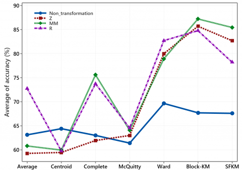
Figure 13. Average the accuracy of six data sets with several clustering methods and transformation

Figure 12 shows the average clustering accuracy of five data sets based on several clustering methods for standardized and non-standardized. According to Figure 12, the clustering accuracy can increase by implementing of three ways transformations.

Pre-processing with transformation can increase accuracy by an average of 10.78%. The highest average increase in accuracy occurred in HD Case 2 data, which reached 18.96%. The lowest average increase in accuracy occurs in breast cancer data, which is 5.45%. In the five datasets, the transformation method based on the ranking of the data in Eq. (3) is slightly higher than Eq. (4). Both transformation methods are higher than Eq. (2).

Figure 13 shows average clustering accuracy for several clustering methods with three standardization using different datasets. Although it is less relevant to calculate the average accuracy of other datasets, Figure 13 shows that standardized data can improve the clustering accuracy. The Ward, Block-KM, and SFKM have similarities in determining the group's centre, namely considering the combination of objects that produce the smallest total deviation in the group. Meanwhile, the hierarchical method with average, centroid, complete and McQuitty linkage works based on the proximity matrix and does not consider the total deviation in the group.

Ward's method produces the highest average accuracy compared to other hierarchical methods. At the same time, the SFKM method cannot apply to zoo data or HD case 2 data which are transformed based on ranking. Thus, the Block-KM is the most suitable partitioning method for the five data sets. The proposed new method applies to all data types. The average clustering accuracy for data without or with standardization is higher than other methods relatively. In general, according to Figure 8 to Figure 14, we conclude that pre-processing via transformation can increase clustering accuracy.