Bagus Wahyudi* | Hangga Wicaksono
© 2022 IIETA. This article is published by IIETA and is licensed under the CC BY 4.0 license (http://creativecommons.org/licenses/by/4.0/).
OPEN ACCESS
Learning media is very importance tools to achieved the learning outcome like capable to design reliability engineering system (RES). The students should be understanding with basic theory of reliability and also have technical skill based on need analysis. Unfortunately, the RES learning media are still not available specially to implement of several type of reliability system. Objective of the study is introducing reliability device model simulation with choice option series, parallel and combine series-parallel system. Method of the study are using accelerated life testing method (ALT) which has been analyzed with statistical method to estimate life-time at normal condition. Validating value of each reliability system are have similarity between experimental test (Re) and theoretical (Rt) i.e.: series (Rt=0.329; Re=0.359); parallel (Rt=0.976; Re=0.972.), and combined of series-parallel (Rt=0. 651; Re=0.686). The conclusion is the parallel have high-fidelity on application of reliability simulation with error 0.000409.
accelerated life test (ALT), reliability, bohlamp, learning media, Weibull distribution
Since 21st century, the commercially available computers have increased significantly both increasingly in higher demand and in affordability. This led to the emergence of the highly sophisticated simulation software applications that do not only enable high-fidelity simulation of dynamic systems, but also automatic code generation for application in industrial controllers. The simulation tools have been broadly used for the design and the improvement of electrical systems since the middle of the twentieth century [1]. The highly sophisticated reliability simulation software applications also provide in software store with several brand such as: CASRE (Computer-Aided Software Reliability Estimation) and an open source SFRAT (Software Failure and Reliability Assessment Tool), Visual-XSel 12.0, Minitab Reliability Expert Support, and Weibull ReliaSoft's for reliability.
This paper discusses the idea of a Learning Media Simulation tool for system reliability engineering subjects. As we know that it is difficult for a teacher to achieve the learning outcomes (LO) on the reliability of systems engineering courses to fit with the realities of factory production, considering that the LO requires investment, time, and resources are expensive. In general, data retrieval life (lifetime) and life characteristics of a product, system or component are done in normal operating conditions [2]. For various reasons, data retrieval by this method may produce difficulties and even impossible to do. The difficulty can be due to increasing longevity of a product at present, the period between designs [3], and shorter product launches, as well as challenges to test the product continuously in normal conditions [4].
We watch the difficulties and the need to find out the failure of the product in order to better understand the failure modes and life characteristics of a product, the analyzer reliability have been trying to create a method so that a product can fail in a shorter time [5]. In other words, practitioners have tried to accelerate the failure of a product. Accelerated life testing involves the acceleration of failure with one goal is to measure the life characteristics of a product under normal conditions.
This research will be tested if there is a significant difference between the theoretical manual calculations with experimental simulation-based equipment reliability. We will to know if the test hardware simulation equipment is no significant difference, then these simulations can represent real equipment at the plant for testing the system reliability. Life testing under nominal operating conditions of mechanical component with high mean lifetime between failure (MTBF) often consumes a significant amount of time and resources [6].
The objective of this research is to know: (1) the reliability value of the bohlamp installation for: series, parallel, and series-parallel based on theoretical calculation and experimental, (2) percentages of reliability value error, (3) to find the best of fidelity simulation test based on model installation that applied. This paper focuses on material that is required for the practical application of simulation reliability; procedure operation, part of system or specimen, collecting data and method of analysis. Although many sophisticated reliability simulation software has been providing in the market but it’s not sufficient to applied in the real practice. There are still required the simulation based on Hardware to achieve the best learning outcome. This study introduces the simple tool ware of reliability engineering model that easy to duplicate.
We studied several researches which have related with learning media i.e.: Grant J S promoting feedback by using the video to improve student which desirable for clinical behaviors in a simulated environment shows high-fidelity [7]. Chronister also says that debriefing before following clinical nursing simulation plays a critical role in achieving student learning outcome [8]. Even a simulation of mechanical transmission system successfully patented which can be used as a human-computer task force and being a feedback interface device connected to a host computer which had a high-fidelity precision [9]. This, in turn, required an analysis tool that able to predict the behavior of electronic components to predict product reliability and identifying when to undertake maintenance, both during qualification testing or maintenance assessment [10].
Falahati studied direct interdependencies inside cyber-power networks and proposed the state mapping-based model to evaluate its impact on the power system reliability [11]. Aghili shows how the purpose of Substation Automation System can respond to the variations in reliability data [12]. Some agenda has been proposed here to support the continuation of the work towards more applications in relation with electric power machinery or systems. Hu shows the need for a probabilistic approach to reliability predictive that took the effects of design variations [13]. Moreover, discussed are technologies for calculate the remaining life of the wrap up when subjected to qualification stresses or in service stresses using prognostics methods. Experiments on reliability engineering using Accelerated Life Testing methods have applied by many researchers, among others: Han and Narendran writing paper with title "An accelerated test method for predicting the useful life of an LED driver" [14]. Chandra and Khan also writing "Optimum plan for step-stress accelerated life testing model under type-I censored samples" [15]. Zhang et al. also develops accelerated life test model using extrapolating data based on accelerated testing to the stress levels within the range (or outside of the range) of testing can effectively evaluate the life probability of a bearing [16].
Reliability assessment also being concern many researchers, among others: Zhang et al. reviews about the state-of-the-art technologies for evaluating the reliability of large-scale PV systems and the effect of PV interconnection on the reliability of local distribution system [17]. Zini et al. shows a procedure for reliability assessment of grid-connected large-scale photovoltaic systems [18]. Ahadi using the fault tree method with an exponential probability distribution function to evaluate the modules of large-scale PV systems [19]. Aval using the Markov method based on the state-space analysis to study the impacts of implementation of BCHP systems on the power systems’ reliability. The Markov method is very well for analyze the reliability of systems based on a continuous stochastic process [20]. Hayati et al. proposed a new procedure for reliability assessment-based substation and distribution automation considering secondary device faults to improve reliability of an IEC 61850 [21]. Lei and Singh studied the quantitative relationship between switching time and system-wide energy unavailability, they present a systematic methodology for considering the effect of cyber-malfunctions in substations on power system reliability [22]. Wang et al. introduce the Bayesian method to integrate the Accelerated Degradation Testing (ADT) data from laboratory with the failure data from field. Calibration factors are set up to minimize the difference between the lab and the field conditions so as to predict a product's actual field reliability more accurately [23].
In recent years, the phrase "accelerated life testing" has been used to describe the activities as mentioned in related works above. Specifically, accelerated life testing can be divided into two areas: (1) qualitative accelerated testing and (2) quantitative accelerated life testing [24, 25]. In qualitative accelerated testing, engineers are more interested in identifying failures and failure modes without trying to make any predictions of life of the product under normal conditions. In quantitative accelerated life testing, engineers interested in the life prediction of products (MTBF) under normal operating conditions is based on data obtained from accelerated life testing. In most products, components or systems are expected to carry out its function for a long time (many years). In order for companies to be more competitive, the time required for data retrieval time-to-failure must be shorter than expected product life. Two methods have been created to speed up the data retrieval process time-to-failure is accelerating the rate of usage (usage rate acceleration) and acceleration loads more (overstress acceleration). For products which under normal conditions are not used continuously, accelerating the process can be done by continuously using the product. This process is called accelerated rate of use. If the acceleration of the rate of use cannot be used practically on a product, it can have the test by providing loads exceed the specifications of the product under normal conditions. This process is called acceleration with over-loads.
For products which under normal conditions are not used continuously, the product will fail early if the product is used continuously. For example, if a microwave oven operates only for a few hours in the day, the test in the microwave can be done by operating the microwave more often to the point of failure. The same thing can be applied to the dishwasher. Suppose the average washing machine usage time is 6 hours per week, testers can reduce test time up to 28 - fold over by operating the dishwasher continuously. Data obtained from the acceleration of the rate of use can be analyzed by the same method with a data time-to-failure usual. Accelerating the data usage restrictions of use arise when a product such as computer servers and tools supporting resilient in continuous use. In such cases, the examiner should trigger the failure of a product by giving a load (stress). The testing process is referred to overstress acceleration.
For products with a high level of continued use, the examiner must then to create the conditions that can lead to failure of the products tested. This can be achieved by including a load (or several load) exceeding the limit of which can be covered by a product based on normal specifications. Data time-to-failure which can be obtained from this process extrapolate to obtain the life of the product under normal conditions. Accelerated life tests can be done with the temperature, humidity, voltage, pressure; vibration exceeds the limit operation of the product in order to speed up the process of product failure. Testing can also be done by combining various elements above.
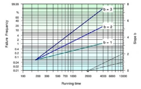
Today, the Weibull distribution is also used in some other applications such as determining the distribution of wind speed at the wind power plant design. Publication of Weibull distribution at first caused debates and opposition. However, at present, the Weibull distribution is used as an industry standard. This study gives special attention to statistical methods, especially methods formulated by Weibull. "The characteristics of the life" and "probability of failure" predetermined from a particular component can be derived from Weibull plot. Probability Density of Failure on the S - Weibull distribution is represented by:
$H=1-e^{-\left(\frac{t}{T}\right)^b}$ (1)
Figure 1. Probability density S at several values of b [26]
S- curve used as a straight line (linearized best-fit straight line) through ordinate scale distortion (double logarithmic) and abscissa (logarithmic) as shown in Figure 1. The advantage of this method is increasingly easy to identify whether any such distribution Weibull distribution or not. Other than that, reading the value on the plot becomes easier. The slope of the curve in Figure 2 is determined as a direct function of the curve parameter b, therefore, the addition of scale to b often given to the right of the plot. The slope can be determined graphics by sliding a straight line parallel through "poles" (on the x-axis to 2000 on the plot).
Figure 2. Simplification of the probability density curve [26]
The reliability value is often used as a substitute for the frequency of failure value:
$R=e^{-\left(\frac{t}{T}\right)^b}$ (2)
$R=1-H$ (3)
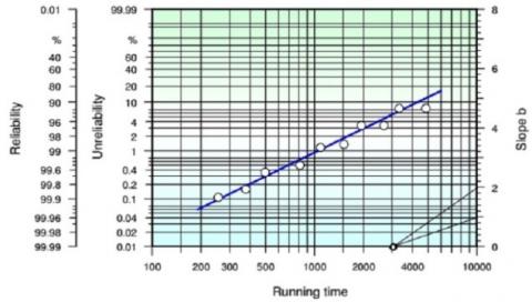
The equation above shows how many components can still be used after reaching a certain time or that have not failed. (Y-axis in the plot Weibull read from top to bottom as seen in Figure 3):
Figure 3. Probability Density with Y axis as a marking scheme of reliability [26]
The series system is a configuration whereby if there is one component fails then the whole system will fail. In concept, the series configuration system (See Figure 4) is a system that has the same drawback with the composition of the weakest, [27].
Figure 4. Series configuration system
If each reliability component has different value:
RS=R1×R2×…Rn (4)
If each reliability component has similar value:
$R_S=\left[R_i\right]^n$ (5)
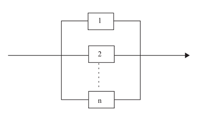
The parallel system is a configuration during which not all the components fail if one of parts fail so the system can still work. In concept, the parallel configuration system (Figure 5) is not influenced by one-part fail and cause failure all system (shutdown) so still has the highest reliability value when compared with others model. Parallel installation can be illustrated in a system with 2 pieces of identical parts (n=2). The system can last up operation time T if one or both of the components continue to function (not a failure).
Figure 5. Parallel configuration system
If each reliability component has different value:
$R_s=1-\prod\left(1-R_1\right)=1-\left(1-R_1\right) \times\left(1-R_2\right) x\left(1-R_n\right)$ (6)
If each reliability component has similar value:
$R_s=1-\Pi\left(1-R_1\right)=1-[1-R]^n$ (7)
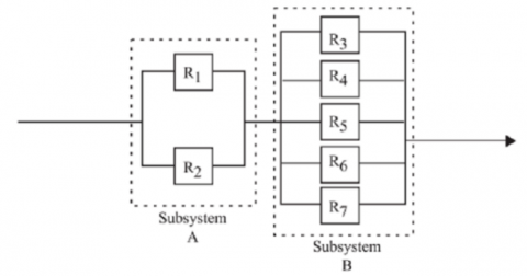
The combined series-parallel system would be explained on configuration Figure 6. Example: The first subsystem consists of two blocks of identical components are arranged in parallel and the second consists of five blocks are also arranged in parallel. Next, merge the two subsystems into one system and calculate the value of the reliability of the overall system.
Figure 6. Configuration of combine series-parallel system
In general, the life of the bohlamp is defined as the period between the first ignitions to the point where the bohlamp fails to emit the light. Bohlamp life is a function of how fast the pitch evaporation of the tungsten filament. It can result from a variety of factors, among others, the type of light, color temperature, duty cycle, and qualification of use.
The changes in the voltage can affect the changes in the properties of light, among others, changes in currents, and power of irradiation. Three changes of the property above can be estimated by using Eq. (8):
Rerated Life $=\left[\frac{V_d}{V_a}\right]^d \times$ Life at Design Voltage (8)
where, Vd=Design Voltage (Voltage from manufacture); Va=Applied Voltage (Voltage applied to bohlamp); d=Exponential based on lamp type.
Median rank used to obtain the estimation of the unreliability of each failure. This value indicates the probability of failure of the actual value of the failure j from a sample of N components with a confidence level of 50%. This essentially means that the method is the best estimate for unreliability: with the possibility of 50% above the true value or below the estimated value. Such estimates were processed through a binomial distribution.
Stapelberg [27] introduce Bernard approximation method is a method for finding the median rank approach to the equation:
$M R=\frac{j-0.3}{N+0.4}$ (9)
where, MR=Median Rank; j=Rank of failure N; N=Number of specimens.
In a linear regression, it can be estimated that the graph ln (cycles) vs. transformation median rank develops into linear mode, because the cumulative Weibull distribution can be transformed become straight line through the equation Y=mX+b.
The following is the derivative of the formula:
$F(x)=1-e^{-\left(\frac{x}{\alpha}\right)^\beta}$$1-F(x)=e^{-\left(\frac{x}{\alpha}\right)^\beta}$$\ln (1-F(x))=-\left(\frac{x}{\alpha}\right)^\beta$$\ln \left(\frac{1}{1-F(x)}\right)=\left(\frac{x}{\alpha}\right)^\beta$$\ln \left[\ln \left(\frac{1}{1-F(x)}\right)\right]=\beta \ln \left(\frac{x}{\alpha}\right)$$\ln \left[\ln \left(\frac{1}{1-F(x)}\right)\right]=\beta \ln \mathrm{x}-\beta \ln \alpha$ (10)
By comparing this equation with a simple equation of a straight line, it is known that the left side of the equation can be equated with the Y, ln X can be equated with X, β can be equated with m, and – β ln α can equated with b. Such that when a linear regression carried out, the estimation of Weibull parameters β is derived directly from the slope / gradient of the line. Estimates for the parameter α should be calculated as follows:
$\alpha=e^{-\left(\frac{b}{\beta}\right)}$ (11)
Weibull line parameter β indicates whether the failure rate will be increasing, constant, or decreasing. Value of β<1.0 indicates that the product has a reduced failure rate. This scenario as distinctively early damage "infant mortality" and indicates that the product fails during the period of "burn-in". Value of β=1.0 indicates that the failure rate is constant.
Usually, it is found that the components which survived from burn-in process will show the value of a constant failure rate. Value of β>1.0 indicates increased failure rate. This happens especially in components that receive friction forces cause wear as happened in parts of the journal bearing having value of β>1.0.
Weibull life characteristics symbolized by α, is a measure of scale in distribution data. Based on the data, it was found that the value of α is the value at which 63.2% of the product cycle has failed. In other words, for the Weibull distribution R (α=0368, regardless of the value of β). For example, about 37% of the bearing journals supposedly will survive for at least 693.380 cycles. To determine which design has a value higher reliability in the cycle to 400, 000 would require the reliability formula, as follows:
$R(t)=e^{-\left(\frac{x}{\alpha}\right)^\beta}$ (12)
By substituting some variables that have been available, can determine the reliability of the estimated value of each design:
$R(400.000)_{\text {Design } A}=e^{-\left(\frac{400.000 \quad}{693.380}\right)^{4.25}}=0.908$
$R(400.000)_{\text {Design } B}=e^{-\left(\frac{400.000 \quad}{723.105}\right)^{2.53}}=0.800$
In a simulation study on the reliability system of bohlamps installation used simulation module installation and accelerated life test (ALT) module testing. Data were collected through two stages: data collection lifetime of ten sample light bulb. The first stage is collecting life data of the bohlamp, whereby the bulb can be estimated lamp life in normal use. The second stage is the life of the bohlamp to process data based on the Weibull distribution using software applications (MS. Excell). Based on the Weibull distribution will be known the value of the reliability of the individual bohlamp. The reliability value is then used for further data processing on wiring installations (by experiment approach) and also theoretically using Eq. (1) until Eq. (12) (by estimation approach).
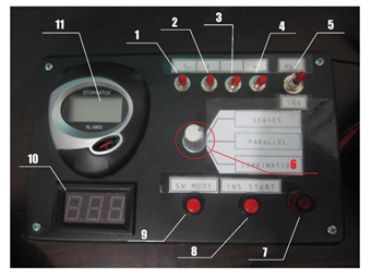
Collecting data on the circuit installation is done by arranging the lamp bulb in the simulation module installation. In this module experimental data taken life of the installation is then processed to obtain the value of the reliability of the system. The reliability value obtained from the experimental installation is then compared with the estimated value of reliability theoretically. Based on the schematic in Figure 10, the main resources in the simulation tool are a power supply unit (PSU) with 24 Volts. Via a selector switch, power source lines split into two options, namely to supply power modules accelerated life testing (ATL) or to supply a series of installations. When we use the PSU to supply the electrical installation, three modes can be selected via the selector switch to the circuit series, parallel or a combined series-parallel.
Figure 7 depicts the mechanism scheme of the reliability testing module. The light sensor is powered by two 9-volt batteries arranged in parallel to drive the two relays. The first relay serves as the driving or stop timer (stopwatch), while the second relay serves as a circuit breaker at the installation. Function the second relay is to enable performance installation system can work on one of the layouts of options series, parallel or a combined series-parallel, although all options are installed in parallel systems.
Figure 7. Mechanism scheme of operating procedure the reliability testing module
Based on data of bohlamp life which is obtained from the experimental setup device as seen in Figures 8 and 9, the life of the bohlamp in normal conditions can be estimated by using the Lamp Rerate (Eq. (8)) shows in the first row on Table 1 that the bohlamp life is 1807 second equal with 0.502 hour; V=12 volt; Vo=24 volt; and d=13.5 (exponential value determined based on bohlamp type and material), the life value of all bohlamps can be estimated using MS Excel software. The graph of the linear regression was obtained by using MS Excel as shown in Figure 10.
The estimation life a single bohlamp is presented in the Table 1.
In the process of data collection of individual bohlamp 12-volt DC which tested their life using ALT module, whereby bohlamp in the module is given double voltage from stress design limits so obtained life bohlamp is much shorter than the normal lamp usage. The result test of configuration series, parallel and combine series-parallel shown in Table 2.
The reliability value of the bohlamp will be known through the Bernard Approximation using equation 9 of Median Rank resulted value in third column on Table 3. Weibull distribution processing in this experiment was calculated and draws graphically using MS Excel software [28]. Data processing carried out by entering the estimated the bohlamp life data to apply in MS Excel become simple linear regression. By using a simple linear regression, will be obtained the linear graph of reliability system. In the graph obtained the value of α (life characteristics) and β (curve parameters/gradient). Data α and β is an element used in the reliability equation so that after these two elements have known, the value of the reliability of the bohlamp will be known [29].
Figure 8. Module (Tool Kit) of reliability simulation system
Note: Always select the installation mode selection (selector switch 6 at Figure 8) in appropriate ways after turning on the sensor. If reversed, the installation will not work as it expected performance.
Figure 9. Interior of bohlamp performance testing chamber
Table 1. Estimated of life in normal condition
|
Specimens |
Accelerated Lifetime (second) |
Estimated Normal Lifetime (hours) |
|
1 |
1807 |
5815.15 |
|
2 |
1486 |
4782.13 |
|
3 |
508 |
1634.81 |
|
4 |
2911 |
9376.95 |
|
5 |
1358 |
4370.21 |
|
6 |
1716 |
5522.30 |
|
7 |
1508 |
4852.93 |
|
8 |
1665 |
5358.17 |
|
9 |
1786 |
5747.57 |
|
10 |
1690 |
5438.63 |
Table 2. Experimental data using ALT
|
Model Installation |
Accelerated Lifetime (s) |
|
Series |
1503 |
|
Parallel |
1389 |
|
Combined Series-Parallel |
1050 |
Table 3 shows the result of Median Rank with Bernard approximation by using Eq. (9) we can see that the expression of the regression equation is:
Colom (e) represented as Y-axis of the graph Weibull distribution.
Colom (f) represented as the X-axis on the graph Weibull distribution.
Table 3. Weibull distribution data processing
|
Life |
Rank |
Median Rank (MR) |
1/(1-MR) |
ln(ln(1/(1-MR))) |
ln (Life Bohlamp) |
|
(a) |
(b) |
(c) |
(d) |
(e) |
(f) |
|
1634.81 |
1 |
0.067 |
1.072 |
-2.664 |
7.399 |
|
4370.21 |
2 |
0.162 |
1.195 |
-1.723 |
8.383 |
|
4782.13 |
3 |
0.260 |
1.351 |
-1.202 |
8.473 |
|
4852.93 |
4 |
0.356 |
1.552 |
-0.822 |
8.487 |
|
5358.17 |
5 |
0.452 |
1.825 |
-0.509 |
8.586 |
|
5438.63 |
6 |
0.548 |
2.213 |
-0.230 |
8.601 |
|
5522.30 |
7 |
0.644 |
2.811 |
0.033 |
8.617 |
|
5747.57 |
8 |
0.740 |
3.852 |
0.299 |
8.657 |
|
5815.15 |
9 |
0.837 |
6.118 |
0.594 |
8.668 |
|
9367.95 |
10 |
0.933 |
14.857 |
0.993 |
9.145 |
Figure 10. Linear regression of weibull distribution
Applied of the linear regression of Weibull distribution graph connected by the red dot marking on Figure 10 shows the trend line equation:
Y=2.2646X+19.776
Numbers 2.2646 on the chart above is showing the value of β in equation reliability. This means that the value of β for bohlamp life calculation based on the experiment is similar with the theoretical data of the expected life in normal operation. The amount of α value obtained through Eq. (11):
$a=e^{-\left(-\frac{19.776}{\beta}\right)}$$\alpha=6201.70$
The value of α indicates that the life characteristics of the bohlamp being tested is 6201.70 hours. By giving the desired time variable with a value of T=4000 hours. Then the value of the reliability of each unit bohlamp at T=4000 hours based on Eq. (12) is:
$R(4000)=e^{-\left(\frac{4000}{6201.70 \quad}\right)^{2.2646}}=0.693$
Reliability calculation based theoretical estimation for each configuration of series, parallel and combined series-parallel with assumption that RA=RB=RC=0.693 described below:
Series: R (4000)=RA x RB x RC=R3=0,6933=0.32994
Parallel: R (4000)=1–(1-R3)=0.97107
Combined Series-Parallel:
R (4000)=RA x (1–(1–RB)(1–RC))=0.628
The bohlamp life data which is obtained by using the Accelerated Life Test, with an increase of stress (24 Volts) and Mean Time of T=0.333 hours (Table 1) without estimated time in normal condition (without Eq. (8)), can be described and calculated with the same procedure of the experimental result of the reliability value as follow:
$R(0.333)=e^{-\left(\frac{0.333}{0.535}\quad\right)^{2.2646}}$
R (0.333)=0.711
Reliability calculation based experimental for each configuration of series, parallel and combined series-parallel with assumption that RA=RB=RC=0.711 described below:
Series: R (0.333)=RA x RB x RC=R3=0.6933=0.359
Parallel: R (0.333)=1–(1-R3)=0.976
Combined Series-Parallel:
R (0.333)=RA x (1–(1–RB)(1–RC))=0.651
Table 4. Comparative reliability between experimentally with alt simulation and estimated life (theoretically)
|
Configuration |
Estimated Life (Theoretically) |
ALT Simulation (Experimental) |
Error |
|
Series |
0.329 |
0.359 |
0.083565 |
|
Parallel |
0.971 |
0.976 |
0.000409 |
|
Combined Series-Parallel |
0.628 |
0.651 |
0.035302 |
As shown in Table 4 above that the result of system reliability is not similar between the theoretical calculation and the simulation using ALT model testing. There are differences in the value of the reliability of the system installation of the series, with the theoretical value of 0.329 and the simulation value of 0.359. The parallel model shows that the reliability system has slightly difference with a value of 0.971 in theory and of 0.976 in simulation. The reliability value differences between theory and simulation are also not too far with a model of combinations, with reliability on theory for 0.628 and 0.651 on simulation. The best configuration of result tested is the parallel system because has minimize error (0.000409) and maximize reliability close with R = 1.00. The similarity of the test results between the bulb circuit simulation and calculations using theoretical formulas on the three types of configurations in series, parallel and combination proves that the Reliability Simulation Test is suitable for teaching aids in learning media. Real-time results from the hardware simulation with accurate and complicated models plays an important role in the engineering design and operation of installation systems.
The simulation model can fulfill its function as an auxiliary learning media of the reliability installation system by applying some components such as the power supply, a light sensor and timer devices. The components are arranged such that the data noted the failure time of each installation configuration. Through the course of the simulation model of the experimental data can be resulted in this study. The parallel arrangement system using ALT module test is the best hardware simulation on the bohlamp circuits can be represented in the real installation on the production utility, i.e.: Pumps Station, Gen Set Power Plant, etc. This arrangement is very cheap and suitable to be applied as a teaching media. Based on the value of reliability discussed above, that the parallel installation configuration shows the highest reliability scores and also high-fidelity with error only 0.000409, followed by combined Series-Parallel model with error 0.035302 and series model with error 0.083565. The comparison results can also be used as an indication that there is a correlation between the theoretical analyses with simulation in practice.
[1] Koziolek, H., Burger, A., Platenius-Mohr, M., Jetley, R. (2020). A classification framework for automated control code generation in industrial automation. Journal of Systems and Software, 166: 110575. https://doi.org/10.1016/j.jss.2020.110575
[2] Cordella, M., Alfieri, F., Clemm, C., Berwald, A. (2021). Durability of smartphones: A technical analysis of reliability and repairability aspects. Journal of Cleaner Production, 286: 125388. https://doi.org/10.1016/j.jclepro.2020.125388
[3] Bakker, C., Wang, F., Huisman, J., Den Hollander, M. (2014). Products that go round: Exploring product life extension through design. Journal of Cleaner Production, 69: 10-16. https://doi.org/10.1016/j.jclepro.2014.01.028
[4] Iraldo, F., Facheris, C., Nucci, B. (2017). Is product durability better for environment and for economic efficiency? A comparative assessment applying LCA and LCC to two energy-intensive products. Journal of Cleaner Production, 140: 1353-1364. https://doi.org/10.1016/j.jclepro.2016.10.017
[5] Chen, W.H., Gao, L., Pan, J., Qian, P., He, Q.C. (2018). Design of accelerated life test plans—Overview and prospect. Chinese Journal of Mechanical Engineering, 31(1): 1-15. https://doi.org/10.1186/s10033-018-0206-9
[6] Wibisono, E., Wahyudi, B. (2017). Reliability module simulation using accelerated life test method. Final Project, Diploma of Mechanical Engineering, Repository of Polinema Library.
[7] Grant, J.S., Moss, J., Epps, C., Watts, P. (2010). Using video-facilitated feedback to improve student performance following high-fidelity simulation. Clinical Simulation in Nursing, 6(5): e177-e184. https://doi.org/10.1016/j.ecns.2009.09.001
[8] Chronister, C., Brown, D. (2012). Comparison of simulation debriefing methods. Clinical Simulation in Nursing, 8(7): e281-e288. https://doi.org/10.1016/j.ecns.2010.12.005
[9] Moore, D.F., Martin, K.M., Rosenberg, L.B., Schena, B.M. (2000). Patent and trademark office. U.S. Patent No. 6,020,875. Washington, DC: U.S.
[10] Bailey, C., Lu, H., Stoyanov, S., Yin, C., Tilford, T., Ridout, S. (2008). Predictive reliability and prognostics for electronic components: Current capabilities and future challenges. In 2008 31st International Spring Seminar on Electronics Technology, Budapest, Hungary, pp. 67-72. https://doi.org/10.1109/ISSE.2008.5276460
[11] Falahati, B., Fu, Y. (2014). Reliability assessment of smart grids considering indirect cyber-power interdependencies. IEEE Transactions on Smart Grid, 5(4): 1677-1685. https://doi.org/10.1109/TSG.2014.2310742
[12] Aghili, S.J., Hajian-Hoseinabadi, H. (2017). Reliability evaluation of repairable systems using various fuzzy-based methods–A substation automation case study. International Journal of Electrical Power & Energy Systems, 85: 130-142. https://doi.org/10.1016/j.ijepes.2016.08.010
[13] Lu, H., Bailey, C., Yin, C. (2009). Design for reliability of power electronics modules. Microelectronics Reliability, 49(9-11): 1250-1255. https://doi.org/10.1016/j.microrel.2009.07.055
[14] Han, L., Narendran, N. (2010). An accelerated test method for predicting the useful life of an LED driver. IEEE Transactions on Power Electronics, 26(8): 2249-2257. https://doi.org/10.1109/TPEL.2010.2095885
[15] Chandra, N., Khan, M.A. (2013). Optimum plan for step-stress accelerated life testing model under type-I censored samples. Journal of Modern Mathematics and Statistics, 7(5-6): 58-62.
[16] Zhang, C., Le, M.T., Seth, B.B., Liang, S.Y. (2002). Bearing life prognosis under environmental effects based on accelerated life testing. Proceedings of the Institution of Mechanical Engineers, Part C: Journal of Mechanical Engineering Science, 216(5): 509-516. https://doi.org/10.1243/0954406021525304
[17] Zhang, P., Li, W., Li, S., Wang, Y., Xiao, W. (2013). Reliability assessment of photovoltaic power systems: Review of current status and future perspectives. Applied Energy, 104: 822-833. https://doi.org/10.1016/j.apenergy.2012.12.010
[18] Zini, G., Mangeant, C., Merten, J. (2011). Reliability of large-scale grid-connected photovoltaic systems. Renewable Energy, 36(9): 2334-2340. https://doi.org/10.1016/j.renene.2011.01.036
[19] Ahadi, A., Ghadimi, N., Mirabbasi, D. (2014). Reliability assessment for components of large scale photovoltaic systems. Journal of Power Sources, 264: 211-219. https://doi.org/10.1016/j.jpowsour.2014.04.041
[20] Aval, S.M.M., Ahadi, A., Hayati, H. (2015). Adequacy assessment of power systems incorporating building cooling, heating and power plants. Energy and Buildings, 105: 236-246. https://doi.org/10.1016/j.enbuild.2015.05.059
[21] Hayati, H., Ahadi, A., Miryousefi Aval, S.M. (2015). New concept and procedure for reliability assessment of an IEC 61850 based substation and distribution automation considering secondary device faults. Frontiers in Energy, 9(4): 387-398. https://doi.org/10.1007/s11708-015-0382-6
[22] Lei, H., Singh, C. (2015). Power system reliability evaluation considering cyber-malfunctions in substations. Electric Power Systems Research, 129: 160-169. https://doi.org/10.1016/j.epsr.2015.08.010
[23] Wang, L., Pan, R., Li, X., Jiang, T. (2013). A Bayesian reliability evaluation method with integrated accelerated degradation testing and field information. Reliability Engineering & System Safety, 112: 38-47. https://doi.org/10.1016/j.ress.2012.09.015
[24] Klyatis, L.M., Verbitsky, D. (2010). Accelerated Reliability/Durability Testing as a Key Factor for Accelerated Development and Improvement of Product/Process Reliability, Durability, and Maintainability (No. 2010-01-0203). SAE Technical Paper.
[25] Klyatis, L.M. (2012). Accelerated Reliability and Durability Testing Technology. John Wiley & Sons.
[26] Bermudez, V., Tormos, B., Olmeda, P., Martin, J. (2008). Spreadsheet for teaching weibull statistical distribution fitting in maintenance engineering. The International Journal of Engineering Education, 24(6): 1210-1216.
[27] Stapelberg, R.F. (2009). Availability and Maintainability in Engineering Design. pp. 295-527, Springer, London.
[28] John, I. (2012). Lamp life accelerated test and validation. https://www.academia.edu/Documents/in/LAMP_LIFE_ACCELERATED_TEST_and_VALIDATION.
[29] Curt, R. (2012). Reliability analysis with weibull. www.crgraph.com.