Nuralhuda Aladdin Jasim* | Manal Abdulsatter Muhammed
© 2022 IIETA. This article is published by IIETA and is licensed under the CC BY 4.0 license (http://creativecommons.org/licenses/by/4.0/).
OPEN ACCESS
The Reynolds number apparatus has been designed. The idea of this device enters all the details of life, all trains, wing of aircraft and ships, and each of them has a specific characteristic. Besides, the Reynolds number apparatus is designed to study the characteristics of fluid such as the velocity of the fluid, discharge, friction factor and the roughness coefficient. (Reynolds number) device was manufactured and fully took all information and details on how to use the device through the lessons given and reliable sources. The results from the device were taken such as the time and the amount of volume in liters. Some types of flow remained in their condition and others changed from transitional flow to turbulent flow. Based on the results, the relation between Reynolds numbers and friction factor are analyzed and the correlation between the time and the discharge are calculated too to investigate the analysis through this apparatus. The results proved all three types of flow and the relationship between Reynolds and friction factor is considered to be in linear regression. The relationship between discharge and flow velocity and Reynolds number is a 'direct' relationship. The increasing in the friction factor has displayed with decreasing in the value of Re. The R2 fit the model with value near to 0.90 or less. Also, the linear model is fit the relation between discharge and time, the increasing in the flowrate showed with decreasing the time. In some cases, the nonlinear fit the model with R2 near to 70 or less.
Reynolds number, friction factor, laminar flow, turbulent flow, transition flow, linear regression, discharge, velocity
In fluid mechanics, the Reynolds number (Re) is a dimensionless number that represents the ratio of inertial to viscous forces, and hence measures the relative importance of these two types of forces under specific flow circumstances.
A flowing fluid's Reynolds number (Re) is derived by multiplying the fluid velocity by the internal pipe diameter (to obtain the fluid's inertia force) and then dividing the result by the kinematic viscosity (viscous force per unit length).
The Reynolds number, abbreviated as Re, is used to determine whether a fluid flow is laminar or turbulent. In technical terminology, the Reynolds number is the ratio of inertial forces to viscous forces. In practice, the Reynolds number is used to predict whether a flow would be laminar or turbulent [1].
The Reynolds Number is the most widely used metric for determining the boundary between laminar and turbulent flow. As the mean velocity of a fluid flow increases and the Reynolds number rises, momentum forces take over [2].
The dimensionless Reynolds number is critical when predicting trends in a fluid's behavior. It is one of the most essential governing parameters in a numerical model for viscous flows [3].
Although the Reynolds number comprises both static and kinematic properties of fluids, it is referred to as a flow parameter because dynamic conditions are investigated. In practice, the Reynolds number is used to predict whether a flow would be laminar or turbulent [4].
If inertial forces, which resist a change in velocity and are the cause of fluid movement, are dominant, the flow is turbulent. A glass of water, for example, is at rest when it stands on a static surface and is unaffected by any forces other than gravity. Flow attributes are ignored. Thus, this results in independence from the Reynolds number for a fluid at rest. When a water-filled glass is tilted, water spills, but flow qualities obey physical rules, and a Reynolds number can be used to predict fluid flow [5].
After attempting to compute drag force on a sphere while ignoring the inertial element, Sir George Stokes (1819-1903) suggested the notion of a dimensionless number that predicts fluid movement.
In 1851, Stokes expanded on Claude Louis Navier's (1785-1836) experiments, establishing the equation of motion by adding a viscous element, revealing the Navier-Stokes equation [6].
"Philosophical Transactions of the Royal Society" published Osborne Reynolds' paper on the dimensionless number, titled "an experimental analysis of the circumstances which decide whether the velocity of water in parallel channels should be direct or sinuous."
The dimensionless number was referred to as parameter: Math 'R' until German physicist Arnold Sommerfeld (1868 – 1951) presented the 'R' number as the 'Reynolds number' at the 4th International Congress of Mathematicians in Rome (1908), when he referred to it as the 'Reynolds number.' Since then, Sommerfeld's term has been used all throughout the world [7, 8].
There are two types of fluid flow regimes to choose from: laminar and turbulent. Transitioning between regimes is a critical topic that is influenced by fluid and flow parameters. As previously stated, the crucial Reynolds number, which varies depending on the physical case, can be characterized as internal or external, depending on the amount of change. However, whereas the Reynolds number for the laminar-turbulent transition may be properly determined for internal flow, it is difficult to do so for exterior flow [9].
Moreover, the Reynold's number is used to anticipate the transition from laminar to turbulent flow, as well as the scaling of similar but different-sized flow scenarios, such as between a wind tunnel model and the full-scale version of an airplane. The capacity to calculate scaling effects and foresee the commencement of turbulence can be used to predict fluid behavior on a larger scale, such as local or global air or water flow, and thus the accompanying meteorological and climatological implications [10, 11].
1.1 Derivation
The Reynolds number is a dimensionless number that determines whether a fluid flow will be laminar or turbulent based on a variety of factors including velocity, length, viscosity, and flow type.
The applicability of the Reynolds number depends on the properties of the fluid flow, such as density variation (compressibility), viscosity variation (non-Newtonian), internal or exterior flow, and so on. The critical Reynolds number is a representation of the value used to define the transition between regimes, which changes based on the flow type and geometry [12, 13].
The viscous behavior of a flow is predicted by the Reynolds number if the fluids are Newtonian. As a result, understanding the physical situation is crucial in order to avoid generating inaccurate forecasts. Transition regimes and internal and exterior flows with either a low or high Reynolds number are the key fields where the Reynolds number can be fully explored. Newtonian fluids are defined as fluids with a constant viscosity. If the temperature remains constant, it doesn't matter how much stress is given to a Newtonian fluid; its viscosity will remain constant. Some examples are water, alcohol, and mineral oil [14].
1.2 Reynolds applications
The uses Reynolds number like many non-dimensional quantities are for the purpose of constructing miniature models of designs for large machines, in order to undergo many tests. For example, if the goal is to build a new aircraft, a prototype of the plane is usually designed first and builds a reasonable-sized wind tunnel to test its performance in all cases [15]. For the scale model to be realistic in terms of test results, the dimensional quantities in the design and in the model must be identical, including the Reynolds number. In the plane example, the air velocity in the tunnel and the size of the miniature plane are chosen so that Reynolds' number remains the same as in reality [16].
1.3 The purpose of the research
It is to design Reynolds number apparatus. The apparatus is utilized to classify the types of flow and to study the characteristics of flow such as velocity, discharges and others. It's also to explain the effect of Reynolds number on the type of flow in tubes, where the dimensional Reynolds number is a crucial number for classifying the flow.
2.1 Introduction
In nature and in laboratory tests, flow can take two different forms: laminar and turbulent. In laminar flows, fluid particles travel in layers, sliding over one another and causing a modest energy exchange. When a fluid has a high viscosity and travels slowly, it is called laminar flow. Turbulent flow, on the other hand, is characterized by unpredictable fluid particle motions and intermixing, as well as a substantial energy exchange throughout the fluid. When the viscosity of a fluid is low and the velocity is high, this type of flow occurs.
The dimensionless Reynolds number is used to classify the flow condition. The Reynolds number Demonstration is a well-known experiment in which dye is introduced slowly and steadily into a pipe to examine flow characteristics.
The flow condition is classified using the dimensionless Reynolds number. The Reynolds number Demonstration is a well-known experiment that involves slowly and steadily introducing dye into a pipe to study flow characteristics.
Fill the reservoir with a dye that is nothing more than colored fluid (typically potassium permanganate solution). The dye should be the same density as water in terms of weight. Keep an eye on the temperature of the water. You can enable a very low rate of flow through a glass tube by partially opening the exit valve [17].
2.2 Theory
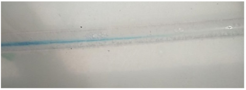
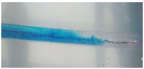
In this experiment, dye injected into a laminar flow produces a clear, well-defined line. It will only combine with the water in a minor way due to molecular diffusion. When the flow is turbulent, the dye will quickly mix with the water due to the substantial lateral movement and energy exchange in the flow.
A transitional stage between laminar and turbulent flows occurs when the dye stream wanders around and shows periodic bursts of mixing, followed by a more laminar behavior [18].
When the dye stream wanders around and shows frequent bursts of mixing, a transitional stage between laminar and turbulent flows occurs, followed by a more laminar behavior.
The Reynolds number (Re) is a helpful metric for describing flow. The Reynolds number is a dimensionless parameter that represents the ratio of inertial (destabilizing) to viscosity (stabilizing) forces. The inertial force grows as Re increases, and the flow destabilizes and becomes entirely turbulent [19, 20].
The Reynolds experiment determines the critical Reynolds number for pipe flow (2000 >Re>4000) at which transitional laminar flow (Re>2000) occurs. The Reynolds number (Re) is a helpful metric for describing flow. The inertial force increases as Re grows, causing the flow to destabilize and become totally turbulent (Re>4000) [21].
The Reynolds experiment establishes the threshold Reynolds number for pipe flow at which laminar flow (Re2000) transitions to transitional flow (2000>Re4000) and transitional flow transitions to turbulent flow (Re>4000) [22]. The application of a critical Reynolds number rather than a critical velocity to all Newtonian fluid flows in pipes with a circular cross-section has the advantage of being universal [23].
The studying the behavior of clustering particles is demonstrated to which it is caused by the acceleration. It is used to understand the behavior of faster natural and artificial phenomena. Also, the application of Reynolds number calculation is studied for the cluster particles [24].
Another application for Reynolds number is found, in which the velocity configuration is performed using Magnetohydrodynamic (MHD) flow. The Reynolds number is calculated in the conditions such as incompressible fluid in pipe section. Some equation was utilized such as Navier-stokes equation, continuity equation, differential equation and finite element method. It was found at the value of Re is equal to 10 and at a x-distance is equal to 0.0034. At numerical results, the velocity increased with the elliptical pipe rather than circular pipe. Thus, the type of cross-section pipe is carried out and it was demonstrated that the elliptical section is more beneficial than circular section using such parameter such as Re [25].
The dimensions of the Reynolds number apparatus are listed as below:
The length of the lowest tank is equal to 150 cm.
The width of the lowest tank is equal to 20 cm.
The height of the lowest tank is equal to 40 cm.
The length of the reservoir tank is equal to 100 cm.
The width of the reservoir tank is equal to 20 cm.
The height of the reservoir tank is equal to 30 cm.
The dimensions of the whole apparatus is considered as 30 cm as the height and the width as 40 cm. The pipe of the glass tube has a diameter of less than 1 inch (22 mm) with the length is equal to 90 cm while the dye injection pipe has a diameter of 1 mm with the length of 20 cm; moreover, it is around of 10 cm enter inside the glass tube and the other 10 cm is considered to be outside the tube. The diameter of the glass tube from the outside is equal to 25 mm and from the inside is equal to 22 mm.
3.1 The procedures for the Reynolds number design
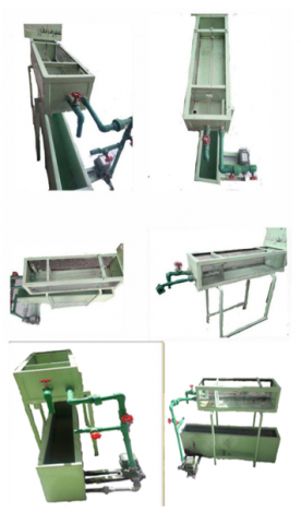
In the designing, we used a plate with the thickness of 2 mm in the upper and lower tanks. The single angle with 6 mm is used to form a border around the glass tank. The glass tank is beneficial to see the flow during the experiment in which the types of flow can be recognized clearly. Based on the lower tank, it is done form plate with 2 mm thickness. The dimension of the lower tank is: 150 cm length, 20 cm width and 46 cm height. While, the dimension of the upper tank is: 100 cm length, 18 cm width, and 30 cm height. Also, the dimension of the table that is hold the upper tank is designed as follow: 60 cm height, 38 cm width. The length of the glass tube is 90 cm with the diameter is equal to 1 inch form outside and 22 mm in the inside. The diameter of the dye injection tube is equal to 3/4 inch. The diameter of the tube connected between two tanks is equal to 1.5 inch. The diameter of the pumping tube is equal to 3/4 inch with control valve in which has the same diameter. The pipes in which connected with the pump are designed in this apparatus is considered to be PPR. In Figure 1, it illustrates the diagram of the Reynold's number apparatus with all its sections. The device consists of a glass tube with a bell mouth entry on one end connected to a constant head water tank and a valve on the other end to control the flow rate.
The flow rate of water is also monitored using a measuring cylinder and a stop watch [26, 27].
Fill the reservoir with a dye (usually potassium permanganate solution) that is nothing more than colored fluid. The dye should have the same weight density as water. Keep track of the water's temperature. By partially opening the outlet valve of a glass tube, you can allow a very low rate of flow through the tube [28].
Figure 1. Reynolds number apparatus
3.2 Reynolds experiment
This paper describes how to perform a laboratory experiment to estimate the critical Reynolds number for a pipe flow under various discharge conditions. The goal of this research is to portray laminar, transitional, and fully turbulent flows in a pipe, as well as the conditions that cause each flow regime to occur.
Flow behavior will also be visualized by pouring dye into a pipe slowly and steadily. Visually determine the flow condition (laminar, transitional, and turbulent) and compare it to the Reynolds number computation findings.
inertial force, Fi= mass * acceleration=density*volume*(velocity/time)=density*area*velocity*velocity
$F_i=\rho \cdot A \cdot v^2\\
F_v=\mu v \cdot D$
where, Fi: inertial force; Fv: viscous force; V: velocity of the fluid; D: diameter.
The Reynolds number is the ratio of inertial and viscous forces in a fluid. The following formula can be used to calculate the inertial force of a fluid:
The Reynold's number is a number that is used to define the flow type. It's a Laminar flow if Re>2000. It's a tumultuous if the number exceeds 4000. In the middle, it's a transition zone. It's also a proportion of inertia and friction." The Reynolds number is a one-dimensional number that indicates whether a fluid flow is laminar or turbulent. Inertial and viscous forces almost entirely drive fluid behavior under dynamic situations [29].
Inertial Force / Viscous Forces = Reynolds number
The fundamental cause of fluid movement that opposes a change in velocity of an item is inertial force.
Resistance to flow is caused by viscous forces.
Turbulent Flow if F inertial is larger than F (force) viscous otherwise, Laminar Flow [18],
$\mathrm{Re}=\frac{F_i}{F_v}=\frac{\rho \cdot A \cdot v^2}{\mu \cdot v \cdot D}=\frac{\rho \cdot v \cdot D}{\mu}=\frac{v \cdot D}{r}$
where, v=velocity of fluid flow, D=diameter of glass tube, ρ=Density of fluid, μ=Dynamic viscosity of fluid, Y=kinematic viscosity of fluid.
In the design the apparatus is required as the following parts:
3.3 Test procedure
The procedure is considered to be as the following:
(1) Adjust the inflow to maintain a consistent head in the supply tank by slightly opening the intake valve. Allow the flow to settle down.
(2) Slowly inject dye and observe its characteristic/behavior.
(3) Determine the amount of outflow.
(4) Increase the discharge by slightly opening the exit valve. Re-establish a steady head in the supply tank.
(5) Repeat steps 1-4 for each discharge until the dye has diffused fully throughout the cross-section of the tube. (Draw a circle around the point at the tube's output end when the dye filament wavers for the first time).
(6) Repeat the experiment with a reduced flow rate, circling the reading where the dye filament wavers for the final time near the tube's output end when the flow changes from laminar to turbulent.
Test procedure of Reynolds experiment is as follows:
Fill the tank with water and let it aside for a while to allow the water to settle.
Fill the tank with water and let it aside for a few minutes to settle the water.
Fill the reservoir with a dye that is nothing more than colored fluid (typically potassium permanganate solution). The dye should be the same density as water in terms of weight.
Keep an eye on the temperature of the water.
A glass tube's output valve can be partially opened to allow a very low rate of flow through the tube.
Once the flow is stable, open the dye injector's inlet valve and let the colored fluid run through the glass tube.
Observe the appearance of dye filament in the glass tube to determine the type of flow obtained for that specific discharge.
Using a stopwatch, keep track of the amount of water gathered in each measurement for a specific amount of time.
Repeat the approach above for changing discharge rates to calculate Reynolds number for each type of flow.
Adjust the flow control valve for a slow trickle outflow, then the dye control valve for a slow flow with a clear dye signal.
The flow volumetric rate is determined via timed water collection.
Observe the flow patterns, take photos, or draw hand sketches as needed to classify the flow regime. Then, using the stopwatch, record different readings for a specific volume of the flow, and then repeat the technique to obtain different readings in order to determine Reynolds number and the fiction factor [30, 31].
You can raise the flow rate by opening the flow control valve. Repeat the experiment to show transitional flow and eventually turbulent flow, which is characterized by continuous and extremely rapid dye mixing as flow rates increase.
A laminar feature can appear in the upper half of the test segment at moderate flows before shifting to transitional flow farther down. The behavior of the upper section is described as "inlet length flow," implying that the boundary layer has not yet extended over the pipe radius.
The temperature of the water is then determined.
Return the remaining dye to its original container to store it. To guarantee that no dye remains in the valve, injector, or needle, completely rinses the dye reservoir [32, 33].
3.4 Observations
Make the following observations while passing colored fluid through a glass tube.
In the three cases below, observe the development or appearance of dye filament in the glass tube at various velocities and record the flow type based on the appearance.
When dye filaments create a straight line, this is known as laminar flow [34, 35].
When dye filament flows in a slightly wavy pattern, this is known as transition flow.
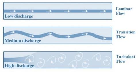
When a dye filament diffuses throughout the whole cross section of a tube while traveling through it, this is known as turbulent flow. All three of these flows are depicted in the diagram below.
The discharge through this pipe is regulated by a control valve and measured with a measuring cylinder.
As a result, the Reynold’s number and flow velocity can both be computed [36, 37].
A dye reservoir sits on top of the head tank, from which a blue dye can be injected into the water to monitor flow.
The dye injected into the water in the head tank is regarded as a sign in our design, allowing flow conditions to be observed. Laminar flow, transitional flow, and turbulent flow are the three types of flow conditions [38]. These types are shown in the Figure 2, Figure 3, Figure 4 and Figure 5.
Figure 2. Types of flows in pipe flow
Figure 3. Laminar flow condition
Figure 4. Transitional flow condition
Figure 5. Turbulent flow condition
In this section, the calculation is done based on the data in which collected based on the Reynolds number apparatus in which is designed. The Tables 1-7 display the calculations for the Re and friction factor for different run of the apparatus.
Table 1. The calculation of Re and friction factor for first term
|
f |
Flow regime |
Re |
Dynamic viscosity |
Velocity) m\s) |
Discharge (m3\s) |
Run |
|
0.033 |
Laminar flow |
1925 |
$1 * 10^{-3}$ |
0.0877 |
$3.333 * 10^{-5}$ |
1 |
|
0.046 |
Transition flow |
2138 |
$1 * 10^{-3}$ |
0.0974 |
$3.703 * 10^{-5}$ |
2 |
|
0.045 |
Transition flow |
2309 |
$1 * 10^{-3}$ |
0.1052 |
$4 * 10^{-5}$ |
3 |
|
0.044 |
Transition flow |
2511 |
$1 * 10^{-3}$ |
0.1144 |
$4.347 * 10^{-5}$ |
4 |
|
0.044 |
Transition flow |
2625 |
$1 * 10^{-3}$ |
0.1196 |
$4.545 * 10^{-5}$ |
5 |
Table 2. The calculation of Re and friction factor for second term
|
f |
Flow regime |
Re |
Dynamic viscosity |
Velocity (m\s) |
Discharge (m3\s) |
Run |
|
0.042 |
Transition flow |
3038.71 |
1*10-3 |
0.1384 |
5.26*10-5 |
1 |
|
0.033 |
Turbulent flow |
4105.77 |
1*10-3 |
0.187 |
7.14*10-5 |
2 |
|
0.035 |
Transition flow |
3381.224 |
1*10-3 |
0.154 |
5.88*10-5 |
3 |
|
0.035 |
Transition flow |
3842.3 |
1*10-3 |
0.175 |
6.66*10-5 |
4 |
|
0.034 |
Transition flow |
3842.3 |
1*10-3 |
0.175 |
6.66*10-5 |
5 |
Table 3. The calculation of Re and friction factor for third term
|
f |
Flow regime |
Re |
Dynamic viscosity |
Velocity )m\s) |
Discharge (m3\s) |
Run |
|
0.069 |
Laminar flow |
922.152 |
1*10-3 |
0.042 |
1.6*10-5 |
1 |
|
0.062 |
Laminar flow |
1031 |
1*10-3 |
0.047 |
1.81*10-5 |
2 |
|
0.091 |
Laminar flow |
702.59 |
1*10-3 |
0.032 |
1.25*10-5 |
3 |
|
0.032 |
Laminar flow |
1976.04 |
1*10-3 |
0.090 |
3.44*10-5 |
4 |
|
0.091 |
Laminar flow |
702.59 |
1*10-3 |
0.032 |
1.25*10-5 |
5 |
Table 4. The calculation of Re and friction factor for fourth term
|
f |
Flow regime |
Re |
Dynamic viscosity |
Velocity )m\s) |
Discharge (m3\s) |
Run |
|
0.033 |
Turbulent flow |
4443 |
$1 * 10^{-3}$ |
0.2024 |
$7.692 * 10^{-5}$ |
1 |
|
0.032 |
Turbulent flow |
4814 |
$1 * 10^{-3}$ |
0.2193 |
$8.333 * 10^{-5}$ |
2 |
|
0.032 |
Turbulent flow |
5251 |
$1 * 10^{-3}$ |
0.2392 |
$9.0909 * 10^{-5}$ |
3 |
|
0.031 |
Turbulent flow |
5776 |
$1 * 10^{-3}$ |
0.2631 |
$1 * 10^{-4}$ |
4 |
|
0.030 |
Turbulent flow |
7221 |
$1 * 10^{-3}$ |
0.3289 |
$1.25 * 10^{-4}$ |
5 |
Table 5. The calculation of Re and friction factor for fifth term
|
f |
Flow regime |
Re |
Dynamic viscosity |
Velocity )m\s) |
Discharge (m3\s) |
Run |
|
0.053 |
Laminar flow |
1203 |
$1 * 10^{-3}$ |
0.0548 |
$2.083 * 10^{-5}$ |
1 |
|
0.049 |
Laminar flow |
1282 |
$1 * 10^{-3}$ |
0.0584 |
$2.222 * 10^{-5}$ |
2 |
|
0.171 |
Laminar flow |
374 |
$1 * 10^{-3}$ |
0.0626 |
$2.380 * 10^{-5}$ |
3 |
|
0.043 |
Laminar flow |
1479 |
$1 * 10^{-3}$ |
0.0674 |
$2.567 * 10^{-5}$ |
4 |
|
0.038 |
Laminar flow |
1648 |
$1 * 10^{-3}$ |
0.0751 |
$2.857 * 10^{-5}$ |
5 |
Table 6. The calculation of Re and friction factor for sixth term
|
f |
Flow regime |
Re |
Dynamic viscosity |
Velocity )m\s) |
Discharge (m3\s) |
Run |
|
0.064 |
Turbulent flow |
3293.4 |
$1 * 10^{-3}$ |
0.154 |
$5.88 * 10^{-5}$ |
1 |
|
0.063 |
Turbulent flow |
3600.78 |
$1 * 10^{-3}$ |
0.164 |
$6.25 * 10^{-5}$ |
2 |
|
0.063 |
Turbulent flow |
3842.3 |
$1 * 10^{-3}$ |
0.175 |
$6.66 * 10^{-5}$ |
3 |
|
0.062 |
Turbulent flow |
4105.77 |
$1 * 10^{-3}$ |
0.187 |
$7.14 * 10^{-5}$ |
4 |
|
0.061 |
Turbulent flow |
4808.3 |
$1 * 10^{-3}$ |
0.219 |
$8.33 * 10^{-5}$ |
5 |
|
0.060 |
Turbulent flow |
5774.42 |
$1 * 10^{-3}$ |
0.263 |
$1 * 10^{-4}$ |
6 |
|
0.059 |
Turbulent flow |
6411.15 |
$1 * 10^{-3}$ |
0.292 |
$1.11 * 10^{-4}$ |
7 |
|
0.058 |
Turbulent flow |
7201.56 |
$1 * 10^{-3}$ |
0.328 |
$1.25 * 10^{-4}$ |
8 |
Table 7. The calculation of Re and friction factor for seventh term
|
f |
Flow regime |
Re |
Dynamic viscosity |
Velocity (m\s) |
Discharge (m3\s) |
Run |
|
0.503 |
Laminar flow |
127.03 |
1*10-3 |
0.2634 |
1*10-4 |
1 |
|
0.554 |
Laminar flow |
115.444 |
1*10-3 |
0.239 |
9.09*10-5 |
2 |
|
0.605 |
Laminar flow |
105.78 |
1*10-3 |
0.219 |
8.333*10-5 |
3 |
|
0.4029 |
Laminar flow |
158.82 |
1*10-3 |
0.3288 |
1.25*10-5 |
4 |
|
0.4029 |
Laminar flow |
158.82 |
1*10-3 |
0.3288 |
1.25*10-5 |
5 |
4.1 The discussion of the Reynolds number and friction factor
The relation between friction factor and Reynolds number:
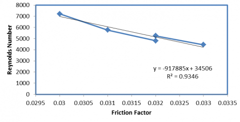
For the first run when the friction factor is laminar, the relation between Reynolds number and the friction factor is expressed as shown in the figure below.
Figure 6. The relation between friction factor and Reynolds Number for the first run
Laminar flow is defined by fluid particles following smooth routes in layers, with each layer moving smoothly behind adjacent layers in fluid dynamics [39].
The fluid tends to move without lateral mixing when mixed at low rates, and the neighboring layers glide behind each other. There are no orthogonal currents in the flow direction, and the fluid has no swirls or swirls.
Fluid particles in laminar flow follow smooth paths in layers, with each layer traveling smoothly after neighbouring layers at moderate speeds with little mixing. Adjacent layers tend to fall behind one another as the fluid flows without lateral mixing.
In the flow direction, there are no orthogonal currents, and the fluid has no swirls or swirls. The shorter the time it takes for the flow to become laminar, the lower the runoff speed.
The relationship between the Reynolds number and the friction factor is seen in Figure 6. The data is fitted using a linear model with an R2 of 0.92.
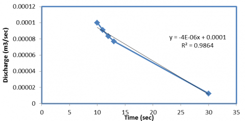
For the second run, the flow became laminar because there were no orthogonal currents on the direction of the flow, and there were no swirls. In laminar flow, and for another reason, a lack of reservoir water results in low pressure. This makes the amount of giants small as time increases, the flow will remain laminar.
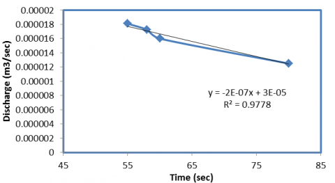
In Figure 7, it illustrates the relation between discharge and time. The linear model is fit the data with R2 is equal to 0.98.
Figure 7. The relation between the discharge and the time for the first run
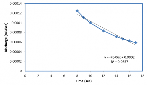
Figure 8. The relation between discharge and time for the second run
Single-phase flow is caused by the difference in pressure between one region and another [1]. Therefore, air minutes move from the high pressure area to the low pressure area to acquire this. The amount of pressure drop is directly proportional to the fluid velocity, and the dimensions and form of the space through which the fluid moves determine the specific kinetic energy of the fluid at a particular velocity [2]. Moreover, in the Figure 8, it demonstrates the relation between the discharge and the time. The linear model is fit the analysis with R2 is equal to 0.993.
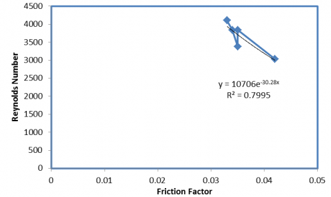
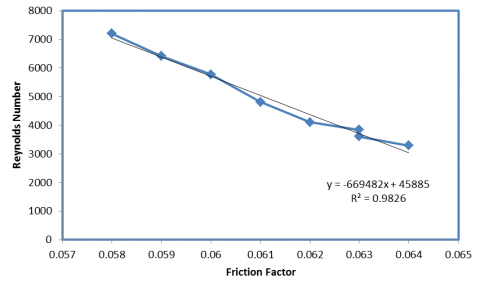
The mismatch between the present results and the reference values in the greatest horizontal velocity defect in the near wake for transient and turbulent flow is most likely due to the plate's limited thickness. At varying Reynolds numbers, the friction coefficient is distributed along the plate's side.
The relationship between Reynolds number and friction factor is seen in Figure 9. The data is fitted with a non-linear model with an R2 of 0.80.
Within the validity range of the latter, the friction coefficient varies on a regular basis. For smaller values of Re, the distribution along the plate does not change considerably, but the pointwise value of the friction coefficient grows more quickly [3].
Figure 9. The relation between friction factor and Reynolds Number for the second run
Figure 10. The relation between discharge and the time for the third run
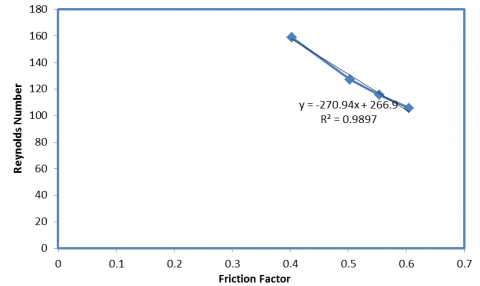
Figure 11. The relation between Reynolds number and friction factor for the third run
Figure 12. The relation between Re and f for the fourth run
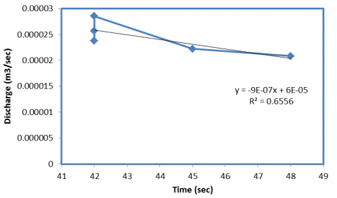
Figure 13. The relation between discharge and time for the fourth run
The longest period of flow was 12 minutes. The flow velocity is shown in Figure 10. The fluid tends to flow without lateral mixing at low speeds, and the adjacent layers glide behind each other. There are no orthogonal currents in the flow direction, and the fluid has no swirls or swirls. The linear model is fitted with an R2 of 0.66.
In Laminar flow, it is occurred in which leads to the confirmation of the quality of the flow and not to divert it to another flow. The Figure 11 represents the relation between Reynolds number and friction factor. The linear model fits the data with R2 is equal to 0.98.
Regarding the fourth run, likewise, for the same previous reason regarding the Reynolds number, the amount of disability is between the fluids and solid particles and the inner walls of the transparent tube decrease when the Reynolds number increases. In Figure 12, it displays the correlation between Reynolds number and friction factor. The non-linear model is fit the data with R2 is equal to 0.98.
In the Figure 13, the relationship between discharge and time is performed. The data fit the linear model with R2 is equal to 0.656. The following criteria have noticed:
For the fifth run, the relation between discharge and time is explained in the figure above. In the Figure 14, it represents the relationship between discharge and time. The linear model is fit the data with R2. The following criteria have been noticed:
Figure 14. The relation between discharge and time for fifth run
Figure 15. The relation between friction factor and Reynolds Number for fifth run
*Shear stress is corresponded with the kinematic viscosity, the lower the Re, the more it will increase. The greater the value of Re, a shear stress inhibitor is proportional to the kinematic viscosity, as it gives positive values.
In the Figure 15, it displays the relationship between the friction factor and Reynolds number. The linear model is fit the data with R2 is equal to 0.53.
For the sixth run as shown in the Figure 16, the relation between friction factor and Reynolds number is shown in the figure above. It is noted that the higher the Reynolds number, the lower the pressure drop value will increase at the same ratio of solid load and this is due to the fact that the flow becomes turbulent.
Figure 16. The relation between friction factor and Reynolds Number for sixth run
Figure 17. The relation between discharge and time for sixth run
More often the greater Reynolds number and this disruption to flow cause an increase in pressure loss (hypotension).
The behavior of the pigment flow layer can be studied in turbulent flow regimes, and the flow control valve at the tube's end was utilized to adjust the speed of the water inside the tube. When the speed was low, the colored layer remained visible along the length of the huge tube. As the velocity was raised, the layer split at a specific spot and spread over the liquid cross section. The transition from laminar to turbulent flow was the location where this occurred.
If we notice the difference between Figure 14 and Figure 17, it is at the highest time of 30 seconds.
The first is laminar flow, and the second is from my lamellar to my disorder. This is due to the difference in flow velocity, which has a major impact on determining the type of flow.
The flow rate depends on the density, fluid velocity, and area of the tube segment. The higher the velocity, density, or area of the tube section is related to the higher the flow rate.
Since the height of the liquid in the tank decreases gradually whenever the amount of the liquid decreases, the speed also decreases and the flow rate decreases gradually, and this means that the liquid exit rate changes with the change of time and therefore it is not correct to calculate the time required to empty the tank by dividing the weight of the liquid by its exit rate, and this is only permissible when the exit rate is constant, in the Figure 18, it indicated the relationship between discharge and the time.
There are several ways for a boundary layer to shift to turbulence. The beginning conditions, such as initial disturbance amplitude and surface roughness, determine which path is physically realized. Each phase has a different level of knowledge.
As it is appeared, the correlation between Reynolds number and the friction coefficient is shown in the Figure 19. It is a non-linear relationship and friction decreases with increasing Reynolds number.
Figure 18. The relation between discharge and time for seventh run
Figure 19. The relation between friction factor and Reynolds Number for seventh run
In fluid mechanics, the Reynolds number (Re) is a dimensionless quantity that can be used to forecast flow patterns in various fluid flow states [5]. Flows prefer to govern laminar flow (paper-like) at low Reynolds numbers, but Reynolds number disruption is caused by variances in fluid velocity and direction, which can sometimes cross or even clash with the flow's main direction (eddy currents). These therapeutic currents begin to flow, consuming energy in the process and increasing the amount of fluid available in the fluid cavities.
Furthermore, the Reynolds number (Re) has a wide range of applications, from fluid flow in a tube to air traveling over a plane's wing. It is utilized in the gradient of comparable but different size flow states, such as between a plane model in a wind tunnel and a full-scale counterpart, to forecast the transition from laminar to turbulent flow. Turbulence forecasts and the capacity to quantify measurement effects can be used to foresee fluid behavior on a larger scale, such as air or water movement on a local or global scale, as well as the climatic and climatic implications that ensue. Although George Stokes invented the notion in 1851, Arnold Somerfield dubbed the Reynolds number after Osborne Reynolds (1842-1912), who was popular in 1883 [6, 7].
In this project, the Reynolds number apparatus has been designed. It is utilized to study the types of flow conditions. Its purpose is to explain the effect of Reynolds number on the kind of flow in tubes, where the dimensional Reynolds number is a critical factor in classifying the flow.
In the manufacturing process, the device was manufactured locally and from different materials, including iron for the upper and lower basin industry, with a thickness of 2 mm, and a separate 6*6 iron was also used to make a frame to hold the side bottle, which gives a real view of the liquid flow process inside the tube and the dye appears clearly, as well as a glass tube with a diameter of 22 Mm for the dye flow into the tube and give the special type of flow. The tube was used for the type of heat-resistant and broken brassite. The material was brought from Baghdad Governorate from special offices for glass bottles. The bottle was installed inside the upper basin with a plastic handle and inserted into the second end of the dye tube. Also, a special pump was installed to raise water from Lower basin to upper basin with a diameter of 3/4 inch tube of type PVC. The tube enters the upper basin and connects to a perforated end to reduce vortices that get to the water currents as a result of raising the water in the pump. These vortices are obtained, as well as the pump is installed next to the basin by iron piers, as well as an iron clip. To make lines and paths for water movement and to prevent disturbances and eddies in the upper basin before entering the transparent tube. Additionally, several readings have been taken in order to study the types of flow phenomena and attain the error of the process in which compared with the R2 value to see whether fit the model or not.
Disturbed laminar transition occurred in the experiment. Experiments with the Reynolds number device, in the boundary layer through a tube, show that the boundary layer becomes stable after a given length of flow. The boundary layer becomes unstable and turbulent when the volume of fluid flowing through the control valve is increased. This instability happens at various scales and with various fluids. In most circumstances, the free current of the fluid velocity outside the boundary layer is considered the flow velocity.
Experimental measurements reveal that for "fully advanced" flows, laminar flow occurs when the return is less than 2300 and turbulent flow occurs when the return is greater than 2900, based on our design for flow in a diameter tube (the diameter is equal to 22 mm). A continuous turbulent flow will form at the lower end of this range, but only a very long distance from the tube's inlet [8]. At unpredictable periods, intermittent flow will begin between the transition from the plate to the turbulence and then back to the plate. This owes to the fluids various velocities and velocities in different sections of the tube's cross-section, which are affected by other factors including tube roughness and flow homogeneity [9, 10].
Furthermore, the laminar flow dominates in the fast-moving tube's core, while the turbulent, slow-moving flow dominates towards the wall. As the Reynolds number climbs and the intermittency between increments rises, the continuous turbulent flow gets closer to the intake, until the flow becomes fully turbulent at a return of > 2900. This result may be used to non-circular channels with a hydraulic diameter, allowing for the determination of the Reynolds transition number for various channel forms. This transmission is also known as Reynolds numbers.
In the laminar flow conditions, in which all the fluid's minutes move along parallel lines inside the tube, and therefore it is also called stratification.
In the turbulent flow regime, in which vortices are formed and the fluid movement becomes random. Mathematically, fluid disturbance is represented by Reynolds decomposition.
Also, when the flow of water turns to the turbulent, that shift requires more energy to push the water than if the flow was flowing, because the turbulent flow causes energy loss due to increased friction with the walls of the vessel - which causes the generation of heat - which changes the viscosity of the water [11, 12].
The relation between the Reynolds number and the friction factor is described in the analysis in which it was found that the relation for some points are considered to be linear relations between discharge and time. As it was known the increasing in the discharge occurred with the decreasing of the time. Also, the decreasing in the discharge happens with the increasing in the time. Thus, the relation is attained to be a linear relationship and the R2 fit the model with value close to 0.90. Thus, the errors in the design are considered to be minor. According to the relation between the Re and f, it was found that there is a correlation between these variables. It was shown with increasing the Re, the value of friction factor decreases and versa visa. The increasing in the friction factor has displayed with decreasing in the value of Re. The R2 fit the model with value near to 0.90 or less. Also, there is a correlation between the discharge and the time. In most cases, the linear model is fit the relation and the increasing in the flowrate showed with decreasing the time. In some cases, the nonlinear fit the model with R2 near to 70 or less. Thus, there is a correlation between the discharge and the time of the experimental recoding data.
Briefly, our design is beneficial in which the various kinds of flow can be studied. Also, it is essential to study the fluid properties such as the discharge, velocity of the fluid, friction factor and the value of the Reynolds number. The observation of different types of flow can be achieved with the Reynolds number apparatus and it can be demonstrated using dye injection through the tube.
In the recommendation part, it might be used different fluid to study the characteristics of the fluid such as viscosity. It is also significant to perform some changes in the design. For instance, the cross-sectional area of the tube is changed for liquid to flow with a surface. Thus, distinctive dimension can be used to give an essential value of Reynolds number to start with the turbulence in the flow of the tube. In some cases, changing the parameters of the width with the length of the glass tube with different values is to acquire the re-transmission and turbulent flows.
It is obvious that the running water through a surface with a movement of small speed [13]. During the tube, the fluid flow in a tube, the fluid layer in contact with the inner surface of the tube is stable. This is an indication of the laminar flow type in a tube. The layers of fluid increase in velocity towards the middle of the tube. Thus, the value of Re reaches the critical value and above, leading to a turbulent movement in the fluid will start due to any imbalance [14].
Based on the analysis, the points are considered to be as the following listed:
1. The ratio of the force of limiting friction and normal reaction between any two surfaces in contact is defined as the coefficient of friction. Angle made with the direction of normal reaction by the resultant of limiting friction force F and normal reaction R. R stands for reaction angle. It is proposed that Re and friction factor be calculated utilizing tow surfaces and the flow properties between them be studied.
2. After executing the tests and taking the relevant measurements, it is recommended that you investigate the amount of pressure inside the tube. Knowing the system's specifications (tube length and diameter, air density, and time) will allow you to extract the following quantities (Re and f). It is suggested that the link between hypotension and flow velocity be shown so that it can be determined whether there is a positive association between flow velocities. The amount of pressure drop in the tube is dependent on the speed of fluid flow into the tube and can be studied.
3. As the flow speed inside the tube increases, the pressure drop increases with Reynolds number.
4. The coefficient of friction has an inverse relationship with flow velocity and Reynolds number [15].
5. The scientists attempted to assess whether turbulence persisted under varied flow conditions by pumping water into the water moving down the pipe to create "turbulent puffs." Turbulence reduces the speed of water flowing out of the pipe's core by roughly 30% while boosting flow speed on the pipe's walls, resulting in water flowing smoothly out of the pipe emerging with a different-shaped jet than turbulent flow, making measurements simple.
6. There is a 'direct' link between discharge, flow velocity, and Reynolds number. The friction factor for a pipe in the transition zone falls fast as the Reynolds number and relative roughness of the pipe decrease. The friction factor line for the smoothest pipe is the lowest, where the roughness ε/D is so minimal that it has no effect.
7. As the Reynolds number increases, the continuous turbulent flow draws closer to the intake and the intermittency between them increases, until the flow reaches Re D> 2900 and is completely turbulent [15].
8. The thickness of the sublayer diminishes as the Reynolds number rises, and so the surface bumps protrude through it. The higher is the roughness of the pipe, the lower is the value of Re at which the curve off vs Re branches off from smooth pipe curve.
To sum up, the study of different types of turbulent flow is suggested in order to see the difference between the rough and smooth turbulent flow. More analysis is needed to study the turbulent flow regime with the roughness of the pipe, thickness of sublayer, relative roughness and others.
This apparatus is designed to assist students in their mechanics lab in which is used later to do experiment for students helping them in their experiments. It was put in the Wasit University to assist students and it is designed as a part of project assessment.
[1] Kolmogorov, A.N. (1991). Dissipation of energy in the locally isotropic turbulence. Proceedings of the Royal Society of London. Series A: Mathematical and Physical Sciences, 434(1890): 15-17. https://doi.org/10.1098/rspa.1991.0076
[2] Almerol, J.L.O., Liponhay, M.P. (2022). Clustering of fast gyrotactic particles in low-Reynolds-number flow. PloS one, 17(4): e0266611. https://doi.org/10.1371/journal.pone.0266611
[3] Adrian, R.J., Marusic, I. (2012). Coherent structures in flow over hydraulic engineering surfaces. Journal of Hydraulic Research, 50(5): 451-464. https://doi.org/10.1080/00221686.2012.729540
[4] Ahlers, G., Funfschilling, D., Bodenschatz, E. (2009). Transitions in heat transport by turbulent convection at Rayleigh numbers up to 1015. New Journal of Physics, 11(12): 123001. https://doi.org/10.1088/1367-2630/11/12/123001
[5] Ahlers, G., Grossmann, S., Lohse, D. (2009). Heat transfer and large scale dynamics in turbulent Rayleigh-Bénard convection. Reviews of Modern Physics, 81(2): 503. https://doi.org/10.1103/RevModPhys.81.503
[6] Araujo, F.F., Grossmann, S., Lohse, D. (2005). Wind reversals in turbulent Rayleigh-Bénard convection. Physical Review Letters, 95(8): 084502. https://doi.org/10.1103/PhysRevLett.95.084502
[7] Hunt, B.R., Sauer, T., Yorke, J.A. (1992). Prevalence: A translation-invariant “almost every” on infinite-dimensional spaces. Bulletin of the American Mathematical Society, 27(2): 217-238.
[8] Barré, J., Mukamel, D., Ruffo, S. (2001). Inequivalence of ensembles in a system with long-range interactions. Physical Review Letters, 87(3): 030601. https://doi.org/10.1103/PhysRevLett.87.030601
[9] Batchelor, C.K., Batchelor, G.K. (2000). An Introduction to Fluid Dynamics. Cambridge University Press. https://doi.org/10.1017/CBO9780511800955
[10] Bensimon, D., Kadanoff, L.P., Liang, S., Shraiman, B.I., Tang, C. (1986). Viscous flows in two dimensions. Reviews of Modern Physics, 58(4): 977. https://doi.org/10.1103/RevModPhys.58.977
[11] Brown, E., Ahlers, G. (2006). Rotations and cessations of the large-scale circulation in turbulent Rayleigh–Bénard convection. Journal of Fluid Mechanics, 568: 351-386. https://doi.org/10.1017/S0022112006002540
[12] Chavanis, P.H. (2002). Statistical mechanics of two-dimensional vortices and stellar systems. In Dynamics and Thermodynamics of Systems with Long-Range Interactions, pp. 208-289. https://doi.org/10.1007/3-540-45835-2_8
[13] Chien, C.C., Blum, D.B., Voth, G. (2013). Effects of fluctuating energy input on the small scales in turbulence. Journal of Fluid Mechanics, 737: 527-551. https://doi.org/10.1017/jfm.2013.575
[14] Corrsin, S. (1961). Turbulent flow. American Scientist, 49(3): 300-325.
[15] Dauxois, T., Holdsworth, P., Ruffo, S. (2000). Violation of ensemble equivalence in the antiferromagnetic mean-field XY model. The European Physical Journal B-Condensed Matter and Complex Systems, 16(4): 659-667. https://doi.org/10.1007/s100510070183
[16] Daviaud, F., Hegseth, J., Bergé, P. (1992). Subcritical transition to turbulence in plane Couette flow. Physical Review Letters, 69(17): 2511-2514. https://doi.org/10.1103/PhysRevLett.69.2511
[17] Guilmineau, E. (2008). Computational study of flow around a simplified car body. Journal of Wind Engineering and Industrial Aerodynamics, 96(6-7): 1207-1217. https://doi.org/10.1016/j.jweia.2007.06.041
[18] Frisch, U., Kolmogorov, A.N. (1995). Turbulence: The Legacy of AN Kolmogorov. Cambridge University Press.
[19] Wang, H., Hawkes, E.R., Zhou, B., Chen, J.H., Li, Z., Aldén, M. (2017). A comparison between direct numerical simulation and experiment of the turbulent burning velocity-related statistics in a turbulent methane-air premixed jet flame at high Karlovitz number. Proceedings of the Combustion Institute, 36(2): 2045-2053. https://doi.org/10.1016/j.proci.2016.07.104
[20] Comte-Bellot, G., Corrsin, S. (1966). The use of a contraction to improve the isotropy of grid-generated turbulence. Journal of Fluid Mechanics, 25(4): 657-682. https://doi.org/10.1017/S0022112066000338
[21] Kim, J., Moin, P., Moser, R. (1987). Turbulence statistics in fully developed channel flow at low Reynolds number. Journal of Fluid Mechanics, 177: 133-166. https://doi.org/10.1017/S0022112087000892
[22] Kweyu, D. (2022). Repercussions of increment in Reynolds number and half distance of major axis on magnetohydrodynamic flow in elliptical pipe. European Journal of Engineering and Technology Research, 7(3): 11-17. https://doi.org/10.24018/ejeng.2022.7.3.2811.
[23] Kweyu, D., Manyonge, A.W., Bitok, K.J. (2021). Velocity profile for magnetohydrodynamic flow in straight horizontal elliptical pipe. Applied Mathematical Sciences, 15: 283-295. https://doi.org/10.12988/ams.2021.994486.
[24] Vallikivi, M., Smits, A.J. (2014). Fabrication and characterization of a novel nanoscale thermal anemometry probe. Journal of Microelctromechanical Systems, 23(4): 899-907. https://doi.org/10.1109/JMEMS.2014.2299276
[25] Sinhuber, M., Bodenschatz, E., Bewley, G.P. (2015). Decay of turbulence at high Reynolds numbers. Physical Review Letters, 114(3): 034501. https://doi.org/10.1103/PhysRevLett.114.034501
[26] Sinhuber, M., Bewley, G.P., Bodenschatz, E. (2017). Dissipative effects on inertial-range statistics at high Reynolds numbers. Physical Review Letters, 119(13): 134502. https://doi.org/10.1103/PhysRevLett.119.134502
[27] Mishra, P., Tripathi, G. (1973). Heat and momentum transfer to purely viscous non-Newtonian fluids flowing through tubes. Trans. Inst. Chem. Eng., 51(2): 141-150.
[28] Monin, A.S., Yaglom, A.M. (2007). Statistical Fluid Mechanics: Mechanics of Turbulence vol 1 (New York: Dover).
[29] Spalart, P., Allmaras, S. (1992). A one-equation turbulence model for aerodynamic flows. In 30th Aerospace Sciences Meeting and Exhibit. https://doi.org/10.2514/6.1992-439
[30] Bernard, P.S., Wallace, J.M. (2002). Turbulent Flow: Analysis, Measurement, and Prediction. John Wiley & Sons.
[31] Spalart, P.R. (2009). Detached-eddy simulation. Annual Review Fluid Mechanics, 41: 181-202.
[32] Spalart, P.R. (1997). Comments on the feasibility of LES for wings, and on hybrid RANS/LES approach, advances in DNS/LES. In Proceedings of 1st AFOSR International Conference on DNS/LES.
[33] Ravelet, F., Marié, L., Chiffaudel, A., Daviaud, F. (2004). Multistability and memory effect in a highly turbulent flow: Experimental evidence for a global bifurcation. Physical Review Letters, 93(16): 164501.
[34] Reynolds, O. (1883). XXIX. An experimental investigation of the circumstances which determine whether the motion of water shall be direct or sinuous, and of the law of resistance in parallel channels. Philosophical Transactions of the Royal Society of London, 174: 935-982. https://doi.org/10.1098/rstl.1883.0029
[35] Roche, P.E., Gauthier, F., Chabaud, B., Hébral, B. (2005). Ultimate regime of convection: Robustness to poor thermal reservoirs. Physics of Fluids, 17(11): 115107.
[36] Pope, S.B. (2000). Turbulent Flows. Cambridge Univ. Press, Cambridge UK.
[37] Saint-Michel, B., Dubrulle, B., Marié, L., Ravelet, F., Daviaud, F. (2014). Influence of Reynolds number and forcing type in a turbulent von Kármán flow. New Journal of Physics, 16(6): 063037. https://doi.org/10.1088/1367-2630/16/6/063037
[38] Torcini, A., Antoni, M. (1999). Equilibrium and dynamical properties of two-dimensional N-body systems with long-range attractive interactions. Physical Review E, 59(3): 2746. https://doi.org/10.1103/PhysRevE.59.2746
[39] Wilkins, G.M., Olmsted, P.D. (2006). Vorticity banding during the lamellar-to-onion transition in a lyotropic surfactant solution in shear flow. The European Physical Journal E, 21(2): 133-143. https://doi.org/10.1140/epje/i2006-10053-9