Ahmad Al-Subhi
© 2022 IIETA. This article is published by IIETA and is licensed under the CC BY 4.0 license (http://creativecommons.org/licenses/by/4.0/).
OPEN ACCESS
Economic dispatch (ED) is one of the most important topics in power system operation and planning. The main purpose of this paper is to develop simple and effective mathematical models for the ED problem. Two stages were considered to solve this problem. First, the ED problem is formulated using linear piecewise functions and then optimally solved using the LP technique at various load values. The effectiveness of the LP in optimally solving the ED problem is verified by applying it to two different test systems. The results are compared with those obtained using other ED optimization techniques. The LP optimization performance of the proposed method is found to be similar to those of the reported techniques. In the second stage, the data collected from the optimization process in the first stage are transferred to TuringBot software. This software is adopted to build efficient mathematical models for the optimal power generation (output parameters) as functions of the load values (input parameters). The main objective of these models is to easily evaluate the optimal power sharing of the generators in an online fashion under rapid variable loading conditions without the need to solve the ED-LP based problem. Optimization techniques, including the LP, generally require considerable simulation times for linearization and optimization code execution, particularly under fast load variations. Thus, the main features of the developed models in this paper are simplicity, accessibility, as well as the ability in obtaining an efficient and optimal solution with a faster execution time.
economic dispatch, TuringBot, linear programming, mathematical models
The economic dispatch (ED) problem is a crucial topic in the field of power system planning and operation. The main objective of the ED solution is to determine the power generated by each generator in order to minimize the total cost while meeting several constraints including load demand and minimum and maximum generation capacity for each generator. An efficient and accurate evaluation of the power generated by each generator can improve the system significantly and lead to a reliable operation of the power system. In recent years, various optimization methods have been proposed to solve the ED problem. The methods differ in different aspects including accuracy, execution time, complexity and simulation workspace. In general, the techniques can be categorized into classical or traditional techniques and heuristic techniques.
Classical techniques have been frequently employed in solving the ED problem. Examples of such techniques include lambda iteration algorithm (LIA), Lagrange multiplier and gradient method. In addition, heuristic and artificial intelligent approaches have been widely adopted for the ED optimization purposes. These techniques include genetic algorithm (GA), tabu search (TS), particle swarm optimization (PSO) and simulated annealing (SA). Other methods include the cost composite function, dynamic programming (DP) and quadratic programming (QP). Moreover, hybrid methods have been also used to solve the ED problem.
A literature survey has recently explored several studies reported on solving the ED problem using both established and new techniques. Examples of such techniques include the gradient method [1], fast lambda iteration (FLA) [2], and enhanced lambda iteration (ELI) algorithm [3].
The PSO is frequently used for ED applications. A thorough literature survey [4] has been conducted on several studies that employed the PSO along with its modified versions to solve the ED problem. Other recent heuristic techniques include the symbiotic organism search (SOS) [5], ant lion optimization (ALO) [6], differential evolution (DE) [7], grey wolf optimization (GWO) [8], flower pollination algorithm (FPA) [9], and gravitational search algorithm (GSA) [10].
Hybrid techniques have been recently employed to optimize the ED problem. A gradient search method with an improved Jaya algorithm has been proposed to solve the ED problem considering environmental issues [11]. Moreover, the bees algorithm (BA) along with the TS has been studied [12], wherein the results were better than those obtained using the general BA. In addition, the hybrid QP and compact formulation method (CFM) have been used for the ED with line losses and prohibited operating zones [13]. Firefly and self-regulating particle swarm optimization (FSRPSO) algorithms are hybridized to solve and optimize the ED problem [14].
The ED problem has been also adopted in the field of Distributed Generation (DG) and smart grids. The objective of ED in the DG field is to optimize the optimal power sharing from different energy sources rather than only one conventional source. Examples of DG sources include wind, solar, battery storage and fuel cell. Thus, adopting such sources add more complexity to the ED optimization model as each DG source has its own limitations and constraints that have to be considered in the optimization process. Various approaches have been proposed to optimize the power generated by different DG systems in smart grid environment [15-17].
In the field of LP, a quick and effective LP algorithm has been applied to solve the ED problem where there are several interconnected micro-grids [18]. Computational experiments demonstrated the accuracy and speed of the LP model [18]. An algorithm to solve the ED problem while integrating renewable energy resources has been described [19]. The algorithm adopts LP owing to its flexibility and reliability. An LP-driven multi-criteria decision making approach has been presented for a multi-objective ED in smart grids [20]. In another study, LP based hybrid method for the ED of both energy and reserve is discussed. Assuming the reserve requirement is evaluated in the optimization process, the technique is used to estimate the optimal power flow and the reserve assigned to each generating unit. This methodology combines LP with two meta-heuristic algorithms: mean-variance mapping optimization (MVMO) and evolutionary particle swarm optimization (EPSO) [21].
In general, the complexity of the ED optimization problem depends mainly on the objective function and the operational system constraints. For example, this would include ignoring or considering transmission line losses. In addition, various other constraints may be added in the problem including the prohibited zone, ramp rate limits, valve point effect, and consideration of environmental issues and carbon emissions. This would add more complexity to the ED problem and more advanced techniques are thus required to find the optimal solution. For example, several studies have analyzed the ED problem in consideration of carbon emissions [22-24]. In addition, the ED problem considering the valve point effect has been also discussed [25, 26].
This high number of research work in this field indicates that this area of study is still under consideration and investigation, and there is still an opportunity to improve the ED optimization process in terms of simplification and accuracy. Although the previously published algorithms have shown efficient performance in solving the ED problem, they are still in need for some requirements. The majority of such algorithms are not easy for anyone to understand. It is not a simple task to understand the algorithm, write the code and tune the parameters and carry out the simulations. Special software programs are also required to perform such simulations. Such programs are usually costly and not easily available in any PC. The main contribution of this work is to develop simple mathematical models that can easily evaluate the optimal power sharing among all generators in very simple and quick way. The models can be easily evaluated without requiring to solve the ED problem. Moreover, the models can be easily implemented in any software such as Excel, MATLAB or any other computational platform.
Another issue in the optimization techniques is the need of solving the ED problem and performing and executing the optimization process at each load value. The actual power systems are usually subjected to rapid load variations. Thus, carrying out the optimization process at each and every load value may increase the simulation time. On other hand, the developed models in this paper can be executed instantly without a need to any iterative algorithms or trial and error operations, hence leading to considerable time saving.
In this paper, all quadratic cost functions are first linearized using piecewise linearized cost functions. After the linearized model is formulated, two ED test systems are solved using the LP optimization model. Accurate mathematical models are then developed using TuringBot software for each generating unit based on the ED simulations and data collected from the LP model. The main objective of such mathematical models is to accurately and rapidly determine the optimal solution under fast load variations without having to solve the ED-LP based algorithm for each load value. The computational analysis in this study was carried out using MATLAB environment on a PC with a 64-bit operating system and a 2.6 GHz processor.
The rest of this paper is organized as follows. Section 2 discusses the ED problem and the linearization approach. Section 3 explains how the general optimization mathematical models are formulated. TuringBot software is briefly presented in section 4. The simulation results and comparative analysis are discussed in section 5 and 6 for the ED-LP based solution and the mathematical models performance, respectively. Finally, the conclusions of this study are given in section 7.
This section discusses the ED problem concept and explains in detail the linearization methodology of the quadratic cost functions of the generators in order to be appropriately used in the optimization process using the LP concept.
2.1 Economic load dispatch problem
The ED problem is an important optimization problem in the area of power generation, operation and planning. In the ED problem, several generating units with their respective cost functions are given. The objective of the ED is to evaluate the produced power by each generating unit in order to minimize the total fuel cost while satisfying the generation-load balance and other technical and operational constraints. In power plants, the ED is considered as a major activity for power system operation and planning for engineers. Therefore, it is highly recommended to accurately estimate the optimal power produced by each generating unit. This can lead to a significant enhancement to the power system reliability.
A typical power plant has several generating units. At any instant of time, the available generating units should be able to meet the total load requirement. The ED optimization process ultimately estimates the optimal power sharing by each generating unit to supply a certain load in the minimum possible cost [27]. Therefore, the objective of the ED optimization process is to find the optimal values of the powers outputted by the generators which will minimize the total cost and satisfy the power demand, units capacity and other operational constraints.
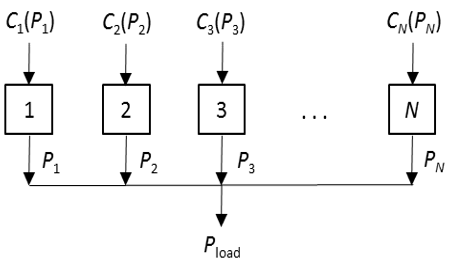
Figure 1 shows the structure of a system composed of N generating units connected to a common bus, supplying a certain load Pload. The input to each unit Ci(Pi) represents the cost of power generation. The output Pi represents the power produced by that unit. The total cost of the system is the summation of the respective generation costs of all units. The first constraint considered here is that the summation of the power generated by each unit must be equal to the supplied load. The second constraint is the generating capacity limits of each unit. These limits define the maximum and minimum powers that can be produced by each unit.
Figure 1. ED problem representation with N generating units
In the optimization process, the objective function Z represents the total cost of the power generated for supplying a given load, while subjected to the defined constraints. Thus, the objective function of the optimization process of the ED problem is represented as follows:
$\text{Minimize }Z=\sum\limits_{i=1}^{N}{{{C}_{i}}({{P}_{i}})}$ (1)
This function describes the relationship between the fuel cost and the power produced by each generating unit. There is one cost function for each unit representing the actual behavior of the generator. In the optimization process, it is required that the power sharing by each generator for supplying a certain load to be accurately optimized such that the fuel cost is minimized.
The cost function usually has the form of a quadratic equation. This function may be also represented by a cubic function for some generating units. Therefore, the quadratic representation of the total cost in $/h for a given generator, i takes the following form:
$C_{i}\left(P_{i}\right)=a_{i}+b_{i} P_{i}+c_{i} P_{i}^{2}, i=1, \ldots, N$ (2)
where, Ci(Pi) is the total generation cost of generator i; ai, bi, and ci are the cost constants of generator i; N is the number of generators; and Pi is the power output of generator i.
The following equality constraint is defined as the power balance equation and is used to impose a balance between the total generation and demand. By ignoring the transmission line losses, this balance is expressed in the form of the following constraint:
$\sum\limits_{i=1}^{N}{{{P}_{i}}}={{P}_{load}}$ (3)
The following inequality constraints are the capacity bounds of the power generator. Each unit i has a lower limit (pi,min) and an upper limit (pi,max) on the power generation. These minimum and maximum limits represent the generation capacity of the generating unit which are related to the technical specifications and design of the generator. These limits are represented by the following constraints:
${{p}_{i,\min }}\le {{P}_{i}}\le {{p}_{i,\max }},i=1,....,N$ (4)
where, pi,min and pi,max are the minimum and maximum power outputs of generator i, respectively.
2.2 Linearization methodology and linear programming
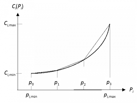
As discussed previously, the cost function presented in (2) is in a quadratic form. Given this nonlinear cost equation for generator i, it is possible to approximate the nonlinear curve by a series of straight-line segments [28]. Figure 2 shows an example of a linearized cost function represented by three linear segments. The linearization methodology has been explained in details in Ref. [28].
For simplicity, in the piecewise linearization approach, the segment widths W are generally considered equal. Therefore, the segment width W can be obtained as follows:
$W=({{p}_{i,\max }}-{{p}_{_{i,\min}}} \quad )/K$ (5)
where, K is the number of segments. Notably, employing more segments will decrease the segment width and improve the linearization accuracy. However, this increases the computation time.
Figure 2. Quadratic cost function linearized by three piecewise linear functions
For generator i, the last point of segment k is evaluated by the following equation:
${{p}_{ik}}={{p}_{i,\min }}+k\times W,i=1,....,N,k=0,....,K$ (6)
where, pi0=pi,min and piK=pi,max.
The linear segment slope, sik is evaluated by estimating the cost values at the starting and end points of a segment (pi,k–1 and pi,k, respectively). Then the difference is divided by the segment width. This is represented by the following equation:
${{s}_{ik}}=[{{C}_{i}}({{p}_{ik}})-{{C}_{i}}({{p}_{i,k-1}})]/W$ (7)
Hence, the cost function for generator i can be re-written as follows.
${{C}_{i}}({{P}_{i}})={{C}_{i,\min }}+{{s}_{i1}}{{P}_{i1}}+{{s}_{i2}}{{P}_{i2}}+....+{{s}_{iK}}{{P}_{iK}}$ (8)
where,
$0\le {{P}_{ik}}\le W,k=1,2,....,K$ (9)
and
${{P}_{i}}={{P}_{i,\min }}+{{P}_{i1}}+{{P}_{i2}}+....+{{P}_{iK}}$ (10)
Therefore, as shown from Eq. (8), this equation is a linear function of the Pik values, which can be optimally evaluated using the LP optimization technique. It is worth to note that the fixed cost constants Ci,min are not considered in the LP optimization process. However, these constants will be added later after solving the optimization problem and evaluating the optimal total cost.
The decision variables in the linearized problem include Pik, where Pik is calculated from the beginning of segment k. For each segment k, the value of the corresponding parameter Pik is obtained as follows.
${{P}_{ik}}=\left\{ \begin{matrix} \min ({{P}_{i}},{{p}_{i,k}})-{{p}_{i,k-1}},\text{ if }{{P}_{ik}}>{{p}_{i,k-1}} \\ 0\text{, otherwise } \\\end{matrix} \right.$ (11)
Several previously reported studies have solved the ED problem in an offline manner. Thus, the ED optimization algorithm was required to be simulated whenever the load changes to determine the optimal solution. Consequently, a longer time is required to solve the ED problem for each load value. Hence, an accurate and simple model is needed to deal with such fast load variations. This section proposes an online dynamic ED model that can be used to determine the optimal solution for any load value without simulating the ED-LP based optimization algorithm.
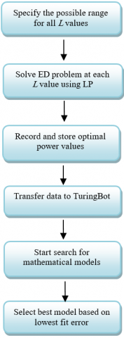
The proposed model is first formulated by considering the generating units shown in Figure 1. This figure shows N generating units with known cost functions required to supply the connected load Pload. Thus, given the range of the load values, the ED problem is solved for each specific load value, wherein the output parameters are the optimal power generated by each generation unit. The proposed LP optimization process is employed to solve the dynamic ED problem wherein the input parameters (load values) and output parameters (optimal power values) are stored and recorded. After finalizing the simulations of the load values, the results are recorded in a table, as listed in Table 1. Here, L1, L2, L3,…., Lnrepresent the load values selected to develop the model (training process). The values must be selected to cover a representative and uniform range of possible connected demands and must be within the range of the sum of the minimum and maximum generator limits.
Table 1. Collected data used to build the general optimization model for each generator
|
Input parameters |
Output parameters |
||||
|
Load (kW) |
Popt1 (kW) |
Popt2 (kW) |
. |
. |
PoptN (kW) |
|
L1 L2 L3 . . Ln |
Popt11 Popt12 Popt13 . . Popt1n |
Popt21 Popt22 Popt23 . . Popt2n |
. . . . . . |
. . . . . . |
PoptN1 PoptN2 PoptN3 . . PoptNn |
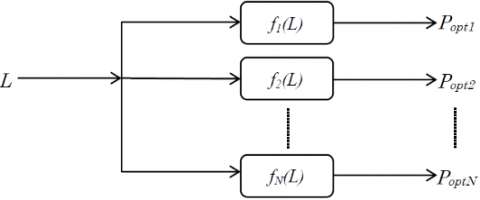
A mathematical model for each generator can be formulated using the data collected and recorded in the table. This model considers the load value as the input parameter and the optimal powers obtained using the LP as the output parameters. The mathematical formulation for each generator takes the following forms:
${{P}_{opt1}}={{f}_{1}}(L)$ (12)
${{P}_{opt2}}={{f}_{2}}(L)$ (13)
${{P}_{optN}}={{f}_{N}}(L)$ (14)
Therefore, each unit has its own optimization model as a function of the input demand. TuringBot software is adopted to build and formulate the mathematical models based on the collected data. Figure 3 shows a flow chart, summarizing the steps followed to build the general optimization model for a selected generator. Figure 4 shows a descriptive block diagram of the general optimization model.
Figure 3. Flowchart of the proposed methodology for general optimization model
Figure 4. Descriptive block diagram of the general optimization model
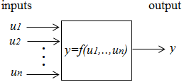
TuringBot is a desktop software that uses symbolic regression to find mathematical models from data values. This software is employed to determine mathematical relationships that describe sets of measured inputs and outputs data in their simplest form [29]. Figure 5 shows the block diagram of the basic function of TuringBot.
Figure 5. Basic function of TuringBot
In this figure, the input parameters, u1….unand the corresponding output parameter y are measured experimentally or by simulations, at which sufficient samples are necessary to represent all operating conditions of the system. The collected input and output data are transferred to TuringBot software to start the training process and formulate the mathematical models. The mathematical relationship representing the output parameter as a function of the input parameters is given as follows.
$y=f({{u}_{1}},{{u}_{2}},.....,{{u}_{n}})\text{ }$ (15)
In TuringBot, different mathematical models are developed and the user can simply select the best model that fits the input/output data with the lowest error.
5.1 Overview
As stated earlier, the proposed ED-LP based algorithm is applied to different benchmark test systems. Two test systems are selected here to carry out this analysis. The first system is a microgrid system consisting of a microturbine and two diesel generators, while the second system is comprising conventional thermal generating units. For each system, the optimal solution for a selected load value is found using the LP and then compared with the values obtained using some other reported techniques.
5.2 Simulation results
5.2.1 DG test system
Three DG systems are incorporated into this system, representing a small microgrid. The cost functions for the DG have the same form as that of the quadratic cost equation of the conventional generators, shown in Eq. (2). Constant parameters values and power generation limits for each DG can be found in the study [30].
The system is discussed here in terms of the ED using the LP for a fixed load value. The quadratic cost functions of the generators are linearized using piecewise linearization as described previously. The problem can then be formulated as a linear equation, which is appropriately used in the LP based model. The MATLAB function linprog is employed to determine the optimal solution to this problem. Table 2 lists the optimal solutions found using the LP for a load value of 200 kW. In addition, the table compares the ED-LP based solutions with some other techniques including the QP using the CPLEX solver and iterated-based algorithm (IBA) [30], LIA [27], and ALO [6].
Table 2. Optimal solution of the three DG system microgrid
|
Load (kW) |
200 |
||||
|
Method |
CPLEX [30] |
IBA [30] |
LIA [27] |
ALO [6] |
LP (proposed) |
|
P1 (kW) P2 (kW) P3 (kW) Total cost ($/h) |
67.949 73.996 58.055
11.076 |
67.96 74 58.03
11.076 |
67.949 73.996 58.055
11.076 |
67.949 73.996 58.055
11.076 |
67.95 73.997 58.053
11.0763 |
5.2.2 Ten thermal units test system
This system comprises ten thermal units having quadratic cost functions. Constants values and generator limits can be found in Ref. [31]. Table 3 lists the optimal solutions to the ED problem obtained using the LP, as well as those obtained using the LIA [27] and ALO [6] for a 2000-kW demand.
Table 3. Optimal solutions of the ten-unit test system
|
Load (kW) |
2000 |
||
|
Method |
LIA [27] |
ALO [6] |
LP (proposed) |
|
P1 (kW) P2 (kW) P3 (kW) P4 (kW) P5 (kW) P6 (kW) P7 (kW) P8 (kW) P9 (kW) P10 (kW) Total cost (\$/h) |
600 600 300 100 50 100 100 50 50 50 16579.75 |
600 599.99 300.01 100 50 100 100 50 50 50 16579.759 |
600 600 300 100 50 100 100 50 50 50 16579.75 |
6.1 Overview
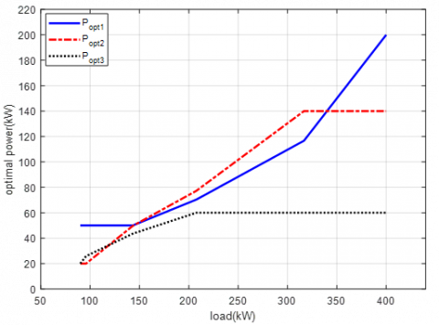
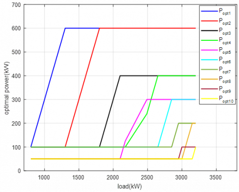
The main objective of this subsection is to formulate accurate mathematical predictive models of the optimal power generated by each unit under variable loading conditions. Therefore, for training data collection, the ED-LP based problem is solved for a wide and representative range of loads. For the DG system, the demand is varied from 90 kW up to 400 kW in steps of 1 kW. For the ten thermal units system, the load is varied from 800 kW to 3200 kW. It should be noted that any load value out of this range gives an infeasible solution, as it would be beyond the sum of the minimum and maximum generator limits. For each load value, the optimal power generated by each generation unit is determined. This process is repeated for all the selected load values and the optimal solutions obtained in each case are recorded and stored. Figure 6 shows the trend in the optimal solutions obtained for each DG with respect to the response to the load variations. Also, for the ten thermal units system, Figure 7 shows the optimal solutions for demand values ranging from 800 kW to 3200 kW, obtained using the same approach as that applied to the three-DG microgrid.
Figure 6. Behavior of the optimal power of each DG under variable loading conditions
Figure 7. Behavior of optimal power of each thermal unit under variable loading conditions
6.2 Simulation results
6.2.1 DG system
From Figure 6, it is clear that some mathematical relationships can be obtained for each parameter as a function of the load demand. A single mathematical model for each parameter can be formulated. However, for more accurate representation, optimal power mathematical relationship can be divided into approximately 4–5 functions based on the load values. Thus, following this arrangement, the final general predictive optimization models for each DG are as shown in Eqns. (16)-(18):
$P_{\text {opt } 1}=\left\{\begin{array}{l}50, \quad 90 \leq L \leq 143.25 \\ 0.3162 L+4.7084, \quad 143.25<L \leq 207.5 \\ 0.4247 L-17.81, \quad 207.5<L<316.75 \\ L-200, \quad \text { elsewhere }\end{array}\right.$ (16)
$P_{\text {opt } 2}=\left\{\begin{array}{l}20, \quad 90 \leq L \leq 95.75 \\ 0.6265 L-40.06, \quad 95.75<L \leq 143.25 \\ 0.4284 L-11.6868, \quad 143.25<L \leq 207.75 \\ 0.5753 L-42.18, \quad 207.75<L<316.75 \\ 140, \quad \text { elsewhere }\end{array}\right.$ (17)
$P_{\text {opt } 3}=\left\{\begin{array}{l}L-70, \quad 90 \leq L \leq 95.85 \\ 0.3735 L-9.9424, \quad 95.85<L \leq 143.25 \\ 0.2554 L+6.9778, \quad 143.25<L<207.58 \\ 60, \quad \text { elsewhere }\end{array}\right.$ (18)
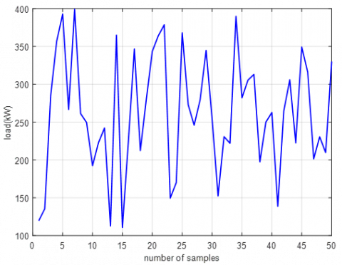
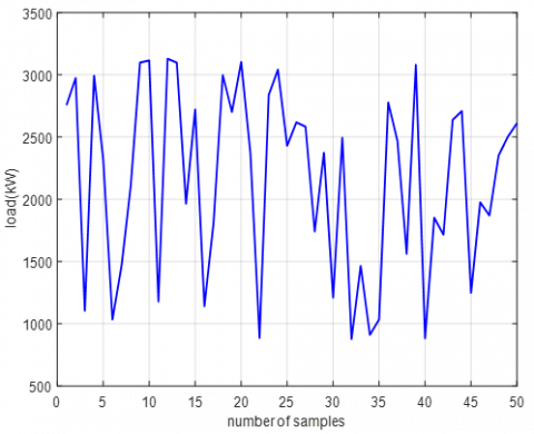
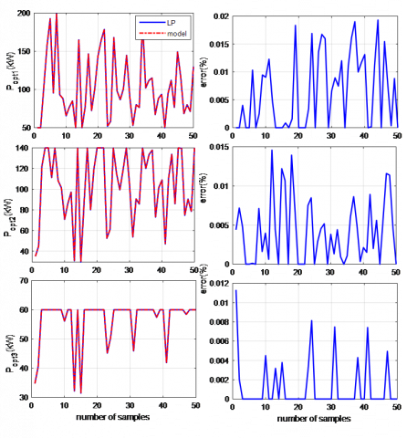
Thus, Eqns. (16)-(18) are employed here to determine the optimal solution of the DG microgrid for any load value within the feasibility range. These equations can be simply coded in MATLAB or any other software to directly evaluate the optimal solution. To check the validity of the developed models, a set of new random load values are used as input variables for both the ED-LP based algorithm and the developed general optimization models. Figure 8 shows 50 new load values selected randomly within the feasibility range.
Figure 8. Randomly generated load profile within the feasibility range of the microgrid
6.2.2 Ten thermal units system
For this system, the general predictive optimization models have been also formulated using the data collected from the ED-LP based simulations. The formulation procedure is the same as that performed for the three-DG microgrid system.
Based on the load variations and by following the solution trend shown in Figure 7, the optimal powers of each generation unit are formulated as a function of the load values as follows:
$P_{o p t 1}=\left\{\begin{array}{l}L-700, \quad 800 \leq L<1300 \\ 600, \quad \text { elsewhere }\end{array}\right.$ (19)
$P_{\text {opt } 2}=\left\{\begin{array}{l}100, \quad 800 \leq L \leq 1300 \\ L-1200, \quad 1300<L<1800 \\ 600, \quad \text { elsewhere }\end{array}\right.$ (20)
$P_{\text {opt } 3}=\left\{\begin{array}{l}100, \quad 800 \leq L \leq 1800 \\ L-1700, \quad 1800<L<2100 \\ 400, \quad \text { elsewhere }\end{array}\right.$ (21)
$P_{\text {opt } 4}=\left\{\begin{array}{l}100, \quad 800 \leq L \leq 2175 \\ 0.4444 L-866.7, \quad 2175<L<2490 \\ L-2250, \quad 2490 \leq L<2650 \\ 400, \quad \text { elsewhere }\end{array}\right.$ (22)
$P_{\text {opt } 5}=\left\{\begin{array}{l}50, \quad 800 \leq L \leq 2100 \\ L-2050, \quad 2100<L \leq 2175 \\ 0.5556 L-1080, \quad 2175<L<2490 \\ 300, \quad \text { elsewhere }\end{array}\right.$ (23)
$P_{\text {opt } 6}=\left\{\begin{array}{l}100, \quad 800 \leq L \leq 2650 \\ L-2550, \quad 2650<L<2850 \\ 300, \quad \text { elsewhere }\end{array}\right.$ (24)
$P_{\text {opt } 7}=\left\{\begin{array}{l}100, \quad 800 \leq L \leq 2850 \\ L-2750, \quad 2850<L<2950 \\ 200, \quad \text { elsewhere }\end{array}\right.$ (25)
$P_{\text {opt } 8}=\left\{\begin{array}{l}50, \quad 800 \leq L \leq 3000 \\ L-2950, \quad 3000<L<3150 \\ 200, \quad \text { elsewhere }\end{array}\right.$ (26)
$P_{\text {opt } 9}=\left\{\begin{array}{l}50, \quad 800 \leq L \leq 2950 \\ L-2900, \quad 2950<L<3000 \\ 100, \quad \text { elsewhere }\end{array}\right.$ (27)
$P_{\text {opt } 10}=\left\{\begin{array}{l}50, \quad 800 \leq L \leq 3150 \\ L-3100, \quad \text { elsewhere }\end{array}\right.$ (28)
Therefore, Eqns. (19)-(28) are used now as general predictive models that can evaluate the optimal solution for any load value without the need to solve the ED-LP optimization problem.
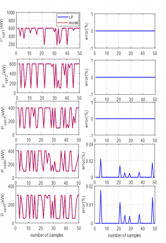
The validity of the proposed models is tested now using some random and new input load values. Figure 9 shows the randomly generated load profile selected from the feasibility range.
Figure 9. Randomly generated load profile within the feasibility range of the 10 thermal units
6.3 Discussion
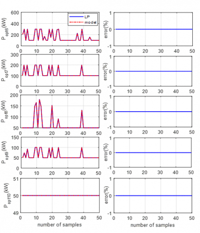
Thus, for both test systems, the performance of the mathematical models in estimating the optimal power generation is compared with the LP solution. Figure 10 shows the comparison of the optimal solutions obtained using both approaches for each DG, including the difference absolute percentage error. Also, Figures 11 and 12 show the comparison between the optimal solutions found using the ED-LP based algorithm and the developed mathematical models for the ten thermal units system. The figures clearly show that the percentage error is very low for all cases, thus verifying the high accuracy of the developed mathematical models and the ability of such models in accurately determining the optimal solutions for any load value within the feasibility range without having to simulate the ED-LP based algorithm.
Figure 10. Optimal solution comparisons between proposed ED-LP based algorithm and the developed general optimization models of the microgrid
Figure 11. Optimal solution comparisons between proposed ED-LP based algorithm and proposed general optimization models for units 1-5
Figure 12. Optimal solution comparisons between proposed ED-LP based algorithm and proposed general optimization models for units 6-10
In this paper, an ED solution methodology is proposed based on the LP concept by linearizing the quadratic cost functions of the generation units. A piecewise linearization is employed, wherein thousands of segments are used to precisely convert the quadratic functions to linear functions. The effectiveness of the methodology is verified by applying it to two different benchmark test systems, and the results are compared with those of other recently reported ED optimization techniques. A general optimization predictive model is then proposed for each generation unit using simple mathematical models, in which the input variable is the load value and the output is the optimally generated power.
The simulations have shown the ability of the developed mathematical models to evaluate the optimal power generation from all generating units. Moreover, simplicity is another feature of the proposed method. Only a few and simple mathematical equations could represent the feasible operating conditions for the selected systems. The models are accessible and easy to be implemented and coded in any software. The models can also be evaluated instantly without performing any complicated algorithms and iterative operations. Thus, the developed models have the features of simplicity, accessibility, accuracy and fast execution time.
[1] Imen, L., Mouhamed, B., Djamel, L. (2013). Economic dispatch using classical methods and neural networks. In 2013 8th International Conference on Electrical and Electronics Engineering (ELECO), pp. 172-176. http://dx.doi.org/10.1109/ELECO.2013.6713826
[2] Zhan, J.P., Wu, Q.H., Guo, C.X., Zhou, X.X. (2013). Fast λ-iteration method for economic dispatch with prohibited operating zones. IEEE Transactions on Power Systems, 29(2): 990-991. http://dx.doi.org/10.1109/TPWRS.2013.2287995
[3] Singhal, P.K., Naresh, R., Sharma, V., Kumar, G. (2014). Enhanced lambda iteration algorithm for the solution of large scale economic dispatch problem. In International Conference on Recent Advances and Innovations in Engineering (ICRAIE-2014), pp. 1-6. http://dx.doi.org/10.1109/ICRAIE.2014.6909294
[4] Abbas, G., Gu, J., Farooq, U., Asad, M. U., El-Hawary, M. (2017). Solution of an economic dispatch problem through particle swarm optimization: A detailed survey-part I. IEEE Access, 5: 15105-15141. http://dx.doi.org/10.1109/ACCESS.2017.2723862
[5] Vedik, B., Naveen, P., Shiva, C.K. (2020). A novel disruption based symbiotic organisms search to solve economic dispatch. Evolutionary Intelligence, 1-36. http://dx.doi.org/10.1007/s12065-020-00506-5
[6] Nischal, M.M., Mehta, S. (2015). Optimal load dispatch using ant lion optimization. Int. J Eng Res Appl, 5(8): 10-19.
[7] Zou, D., Gong, D. (2022). Differential evolution based on migrating variables for the combined heat and power dynamic economic dispatch. Energy, 238: 121664. http://dx.doi.org/10.1016/j.energy.2021.121664
[8] Tung, N.S., Chakravorty, S. (2015). Grey wolf optimization for active power dispatch planning problem considering generator constraints and valve point effect. International Journal of Hybrid Information Technology, 8(12): 117-134. http://dx.doi.org/10.14257/ijhit.2015.8.12.07
[9] Vijayaraj, S., Santhi, R.K. (2016). Multi-area economic dispatch using flower pollination algorithm. In 2016 International Conference on Electrical, Electronics, and Optimization Techniques (ICEEOT), pp. 4355-4360. http://dx.doi.org/10.1109/ICEEOT.2016.7755541
[10] Hota, P.K., Sahu, N.C. (2015). Non-convex economic dispatch with prohibited operating zones through gravitational search algorithm. International Journal of Electrical and Computer Engineering, 5(6). http://dx.doi.org/10.11591/ijece.v5i6.pp1234-1244
[11] Azizipanah-Abarghooee, R., Dehghanian, P., Terzija, V. (2016). Practical multi-area bi-objective environmental economic dispatch equipped with a hybrid gradient search method and improved Jaya algorithm. IET Generation, Transmission & Distribution, 10(14): 3580-3596. http://dx.doi.org/10.1049/iet-gtd.2016.0333
[12] Chansareewittaya, S. (2017). Hybrid BA/TS for economic dispatch considering the generator constraint. In 2017 International Conference on Digital Arts, Media and Technology (ICDAMT), pp. 115-119. http://dx.doi.org/10.1109/ICDAMT.2017.7904946
[13] Wu, Z.L., Wu, Q.H., Zhou, X.X., Li, M.S. (2015). Hybrid quadratic programming and compact formulation method for economic dispatch with prohibited operating zones and network losses. In 2015 IEEE Innovative Smart Grid Technologies-Asia (ISGT ASIA), pp. 1-6. http://dx.doi.org/10.1109/ISGT-Asia.2015.7386963
[14] Nasir, M., Sadollah, A., Aydilek, İ.B., Ara, A.L., Nabavi-Niaki, S.A. (2021). A combination of FA and SRPSO algorithm for combined heat and power economic dispatch. Applied Soft Computing, 102: 107088. http://dx.doi.org/10.1016/j.asoc.2021.107088
[15] Cherukuri, A., Cortés, J. (2017). Distributed coordination of DERs with storage for dynamic economic dispatch. IEEE Transactions on Automatic Control, 63(3): 835-842. http://dx.doi.org/10.1109/TAC.2017.2731809
[16] Huang, B., Liu, L., Zhang, H., Li, Y., Sun, Q. (2019). Distributed optimal economic dispatch for microgrids considering communication delays. IEEE Transactions on Systems, Man, and Cybernetics: Systems, 49(8): 1634-1642. http://dx.doi.org/10.1109/TSMC.2019.2900722
[17] Gil-González, W., Montoya, O.D., Holguín, E., Garces, A., Grisales-Noreña, L.F. (2019). Economic dispatch of energy storage systems in dc microgrids employing a semidefinite programming model. Journal of Energy Storage, 21: 1-8. http://dx.doi.org/10.1016/j.est.2018.10.025
[18] Hoke, A., Brissette, A., Chandler, S., Pratt, A., Maksimović, D. (2013). Look-ahead economic dispatch of microgrids with energy storage, using linear programming. In 2013 1st IEEE Conference on Technologies for Sustainability (SusTech), pp. 154-161. http://dx.doi.org/10.1109/SusTech.2013.6617313
[19] Elsaiah, S., Benidris, M., Mitra, J., Cai, N. (2014). Optimal economic power dispatch in the presence of intermittent renewable energy sources. In 2014 IEEE PES General Meeting| Conference & Exposition, pp. 1-5. http://dx.doi.org/10.1109/PESGM.2014.6939903
[20] Lazzerini, B., Pistolesi, F. (2015). A linear programming-driven MCDM approach for multi-objective economic dispatch in smart grids. In 2015 SAI Intelligent Systems Conference (IntelliSys), pp. 475-484. http://dx.doi.org/10.1109/IntelliSys.2015.7361183
[21] Chamba, M., Ano, O. (2013). Economic dispatch of energy and reserve in competitive markets using meta-heuristic algorithms. IEEE Latin America Transactions, 11(1): 473-478. http://dx.doi.org/10.1109/TLA.2013.6502848
[22] Kuo, M.T., Lu, S.D., Tsou, M.C. (2017). Considering carbon emissions in economic dispatch planning for isolated power systems. In 2017 IEEE/IAS 53rd Industrial and Commercial Power Systems Technical Conference (I&CPS), pp. 1-10. http://dx.doi.org/10.1109/ICPS.2017.7945099
[23] Bhongade, S., Agarwal, S. (2016). An optimal solution for combined economic and emission dispatch problem using artificial bee colony algorithm. In 2016 Biennial International Conference on Power and Energy Systems: Towards Sustainable Energy (PESTSE), pp. 1-7. http://dx.doi.org/10.1109/PESTSE.2016.7516478
[24] Goudarzi, A., Swanson, A.G., Tooryan, F., Ahmadi, A. (2017). Non-convex optimization of combined environmental economic dispatch through the third version of the cultural algorithm (CA3). In 2017 IEEE Texas Power and Energy Conference (TPEC), pp. 1-6. http://dx.doi.org/10.1109/TPEC.2017.7868281
[25] Wu, Z., Ding, J., Wu, Q. H., Jing, Z., Zheng, J. (2017). Reserve constrained dynamic economic dispatch with valve-point effect: A two-stage mixed integer linear programming approach. CSEE Journal of Power and Energy Systems, 3(2): 203-211. http://dx.doi.org/10.17775/CSEEJPES.2017.0025
[26] Bhui, P., Senroy, N. (2016). A unified method for economic dispatch with valve point effects. In 2016 IEEE 6th International Conference on Power Systems (ICPS), pp. 1-5. http://dx.doi.org/10.1109/ICPES.2016.7584108
[27] Wood, A.J., Wollenberg, B.F., Sheblé, G.B. (2013). Power Generation, Operation, and Control. John Wiley & Sons.
[28] Al-Subhi, A.A., Alfares, H.K. (2016). Economic load dispatch using linear programming: A comparative study. International Journal of Applied Industrial Engineering (IJAIE), 3(1): 16-36. http://dx.doi.org/10.4018/IJAIE.2016010102
[29] TuringBot, S. (2021). Symbolic regression software. https://turingbotsoftware.com.
[30] Modiri-Delshad, M., Koohi-Kamali, S., Taslimi, E., Kaboli, S.H.A., Rahim, N.A. (2013). Economic dispatch in a microgrid through an iterated-based algorithm. In 2013 IEEE Conference on Clean Energy and Technology (CEAT), pp. 82-87. http://dx.doi.org/10.1109/CEAT.2013.6775604
[31] Logenthiran, T., Srinivasan, D. (2009). Short term generation scheduling of a microgrid. In TENCON 2009-2009 IEEE Region 10 Conference, pp. 1-6. http://dx.doi.org/10.1109/TENCON.2009.5396184