Mohammad A. Gharaibeh
© 2022 IIETA. This article is published by IIETA and is licensed under the CC BY 4.0 license (http://creativecommons.org/licenses/by/4.0/).
OPEN ACCESS
This paper presents a modified high-accuracy empirical formula for the strain concentration factor in a centrally-placed countersunk holes in isotropic plate under uniaxial tension. Finite Element Method (FEM) was used to investigate the effect of the problem geometric parameters including, plate width and thickness, as well as the hole radius, countersinking depth and angle on the strain concentration factor. The important influence of Poisson’s ratio was also thoroughly discussed. Based on the FEM-generated data and nonlinear regression, a general and high-precision equation for the strain concentration factor was developed. The formulation process was based on producing a general formula for computing the strain concentration factor with unknown coefficients. Such coefficients are determined by minimizing the relative error between the fitted equation and the FE data using nonlinear least squares method. The results of this newly-developed equation were validated with FEA. The comparison showed high accuracy of the present equation in evaluating strain concentration factor in countersunk holes with a relative approximate error of less than 7%. Besides, this equation was efficiently employed to test the various geometric and material parameters on the strain concentration value of countersunk holes. The results of the present equation were compared to the results of older equation available in literature. The comparison proved much higher accuracy of the present equation in evaluating strain concentration factor especially for deeper and larger countersunk holes than the previously published formula.
countersunk hole, strain concentration factor, strain concentration, mechanical design, finite element analysis, tensile loading
In structural engineering, riveting is a very popular joining method of mechanical and structural components such as elastic beams and elastic plates. Countersunk holes are common footprint of rivet which forms geometric discontinuities throughout the thickness of the structure, i.e. plate. This kind of holes generates complicated high stress and strain distributions and produces regions of localized high stress and strain which are commonly referred to as stress and strain concentration regions. An accurate analysis of such high local stresses and strains is very crucial in predicting joint strength and hence fatigue life of the structural member. Stress and strain concentrations are typically measured by the means of stress concentration factor (SCF) and strain concentration factor (SεCF). Such factors are generally defined as the ratio between the maximum stress/strain and the average (nominal) stress/strain values. In fact, several machine design books [1] have insisted on the essential need of reliable strain concentration factor computations, as there are failure theories, such as the maximum strain theory, are mainly focused on the maximum principal strain values in the loaded member. Interestingly, stress concentration factor (Kt) and strain concentration factor (Kt,ϵ) are mathematically related. Specifically, Kt,ϵ=Kt for plane stress and Kt,ϵ=(1-ν2)Kt for plane strain problems, where ν is the Poisson’s ratio of the material of the structure with the stress/strain riser, as proved by Dowling [2].
Stress concentration factors has been widely studied. Pilkey et al. [3], and Savin [4] reported numerous data on the SCF in different stress risers under various loading conditions. Shivakumar and Newman Jr. [5, 6] studied SCF in circular holes drilled in thin and thick elastic plate under uniaxial tension using finite element analysis (FEA). Their studies showed that the stress concentration occurs near the plate edge, in both thin and thick plate systems, perpendicular to the loading direction. However, for thick plates, the high stress localization was found to be at the mid-thickness of the plate and it decays at the top and bottom free surfaces. Another SCF study for plates with central circular drill holes and uniaxial and biaxial tensile loadings was conducted by Mu and Wu [7]. Several research studies in literature for the investigation of SCF in centrally-placed circular holes are available [8-12]. More data on the calculation of SCF in elliptical holes and other types of cutouts is also available [13-16].
For the investigation of SCF and in countersunk holes, only a few studies and papers are available. The first experimental study was performed by Whaley [17]. In which he studies stress distributions at the top and bottom surfaces of the hole instead of its interior. Cheng [18] used stress freezing method to experimentally obtain stresses in countersunk holes through the thickness of the plate. In his study, he considered several countersink depths and angles and two loading conditions: tensile and bending. His stress results showed that the high stress localization occurs at the edge of the countersink. Shivakumar et al. [19, 20] and Bhargava et al. [21] conducted a thorough FEA investigation for the SCF in countersunk holes under remote tension. They also provided empirical formulations to calculate SCF in countersunk holes with different geometric properties. Later, Darwish et al. [22, 23] and Gharaibeh et al. [24] proved that the error in the equations provided by Bhargava et al. [24] is considerably high for thick countersunk hole with large radii and countersink depths. As a result, they provided modified and more accurate equations to compute SCF in countersunk holes subjected to uniaxial tension.
For the SεCF, Chaudhun et al. [25] investigated a long-range elastic strains around circular holes and other discontinuities using X-ray topography methods. Pandita et al. [26] investigated the strain field in orthotropic plates with centrally circular and elliptical holes due to tension using digital photogrammetry. Their results showed that strain concentration values are affected by the loading direction and the holes geometry and dimensions.
Yang et al. [27] used finite element method (FEM) to study stress and stain fields around circular holes in finite thickness large plates. The numerically-simulated results revealed that the stress and strain concentrations occur at the mid-plate of the thickness in thin plates and their location vary in thick plates. Besides, they claimed that the SεCF is often related to Poisson’s ratio; especially for thick plate systems. Ray-Chaudhuri and Chawla [28] investigated the strain concentration in various hole shapes in orthotropic composite plates under uniaxial tension using FEA. The simulation results proved that strain concentrations are highly affected by the shape, size and eccentricity of the hole in addition to the number of plies in the composite plate, fiber orientation and the curvature of the plate. Recently, Ball et al. [29] studied both elastic and plastic stress and strain responses of circular and V-shaped notches in flat plates using FEA and experiments of surface differential displacement mapping. Their results showed that larger and deeper notches end up in higher stress and strain values around the discontinuity. Besides, the investigated the accuracy of their FEA models compared to experimental findings. Zhu et al. [30] proposed a correction factor that includes the effect of Poisson’s ratio effect to quantify the SεCF induced in notched plates using nonlinear finite element computations. Then, they used the results of the new method to fit a high accuracy fatigue life prediction models of TC4 and GH4169 alloyed plates. Guo, W. and Guo, W.L. [31] obtained a complete set of empirical formulas to compute 3D SCF and SεCF in plates with finite thickness having central circular and elliptical holes under uniaxial tension. Additionally, the computations of the empirical formulas were validated with FEA data and other available theoretical solutions in literature. Tlilan et al. [32] introduced a study on the SεCF of thick-walled cylinders with internal pressure. In their study, triaxial as well as biaxial stress states were considered in both open and closed end vessels. The FEA results revealed that the maximum SεCF is located at the inner surface of the pressurized cylinder. Also, the SεCF decreases throughout the thickness toward the outer surface of the pressurized vessel.
For SεCF in countersunk holes, Hayajneh et al. [33] presented strain concentration FEA study in countersunk holes in orthotropic plates under tension. In their FEA models, they adopted two modeling strategies, homogenous modeling and ply-by-ply modeling methods. The results showed that SεCF is function of the hole geometry as well as plate material properties, i.e. Poisson’s ratio. Bhargava and Shivakumar [34] formulated an empirical equation for the SεCF in countersunk holies in isotropic plate subjected to tensile loading based on finite element analysis data. However, it was found that for holes with larger radius and countersink depths in thicker plates, the equations in Ref. [34] are inaccurate and they could lead to erroneous SεCF results.
The objective of this paper is to formulate an accurate equation to compute the strain concentration factor (Kt,ϵ) developed in countersunk holes subjected to uniaxial tension. This proposed equation is more accurate than the equation presented by Bhargava and Shivakumar [34] especially for larger and deeper countersunk holes as the presently proposed equation includes the interaction effect between the hole radius to plate width ratio and the countersink depth which was previously neglected in Bhargava’s work. Specifically, the maximum computed error with respect to FEA data was reduced from 17% to 5%. Therefore, the ignorance of such important effects of the larger and deeper holes could lead to erroneous (Kt,ϵ) values and hence false and extremely dangerous engineering designs.
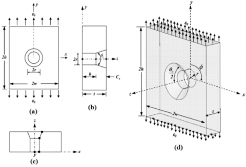
The geometric configuration of a plate with a central countersunk hole is presented in Figure 1. This figure defines the following geometric parameters: The plate length (2h), width (2w) and thickness (t). The plate thickness consists of the straight shank thickness (b) and the sinking depth (Cs), therefore (t=b+Cs). Also, the straight shank radius is (r) and the countersink angle is (θc). In practice, the countersink angle is commonly available in the range of 80°-120°.
In the present analysis, a homogenous, isotropic and linear elastic properties of the Aluminum were used for the plate system with a modulus of elasticity of (E=70 GPa) and Poisson’s ratio of (ν=0.3). For such material configuration, the stress and strain concentration values are independent of E. However, Poisson’s ratio value effects the strain concentration and this effect ranges from 1 for plane stress state to 1-ν2 for plane strain condition.
For a loaded structure, stress and strain concentrations are often defined as the localization of high stress or strain that is results from geometric discontinuities like holes and notches. An accurate analysis of such high local stresses and strains is very crucial in predicting the strength and hence fatigue life of a structural member. Stress and strain concentrations are typically represented by the means of stress concentration factor (SCF) and strain concentration factor (SεCF). Such factors are generally defined as the ratio between the maximum stress/strain and the average (nominal) stress/strain values. Interestingly, stress concentration factor (Kt) and strain concentration factor (Kt,ϵ) are mathematically related. Specifically, Kt,ϵ=Kt for plane stress and Kt,ϵ=(1-ν2)Kt for plane strain problems, where v is the Poisson’s ratio of the material of the structure with the stress or strain riser.
In general, the main focus of this paper is the strain concentration factor (Kt,ϵ) which is mathematically defined as:
$K_{t, \epsilon}=\frac{\epsilon_{\max }}{\epsilon_{\text {nom }}}$ (1)
where, ϵnom is the nominal strain and ϵmax is the maximum strain. In the present configuration, the maximum strain is located at the countersink edge and the nominal strain is equal to the applied strain (ϵo). It is important to mention that both ϵnom and ϵmax in the y-direction, as shown in Figure 1.
Figure 1. Configuration of the countersunk hole: (a) x-y plane (b) y-z plane (c) x-z plane and (d) 3D configuration
In this paper, a comprehensive finite element analysis is performed to investigate the SɛCF in countersunk holes at different countersink angles (θc), thickness to radius ratio (t/r), countersink depth to plate thickness ratio (Cs/t) and radius to width ratio (r/w). To eliminate the influence of the plate length on Kt,ϵ, the plate length to radius ratio is kept constant at (h/r=15) throughout the analysis. Using the FEA data and using nonlinear regression, an empirical formula for Kt,ϵ is developed and hence validated. The formulation process was based on producing a general formula for computing the strain concentration factor with unknown coefficients. Such coefficients are determined by minimizing the relative error between the fitted equation and the FE data using nonlinear least squares method.
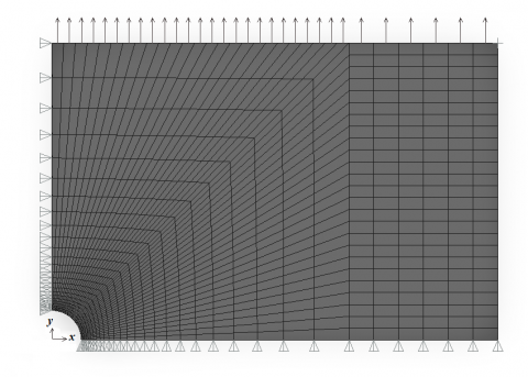
The finite element model of the isotropic plate with a central countersunk hole used in this work was built using ANSYS R17.1. Per the symmetry of the present problem, only one symmetric quarter model was considered. Symmetric boundary conditions were imposed by setting the displacement in x and y directions to zero on x=0 and y=0 planes, respectively. Additionally, the out-of-plane displacement (uz) was constrained at a single node located at x=h, y=w and z=0. A remote strain (ϵo=1) was applied on the x=h plane using INISTATE command available in ANSYS. This quarter symmetric model is shown in Figure 2.
For the FEA mesh design, only three-dimensional hexahedron elements, defined as SOLID185 in ANSYS, was adopted to generate the mapped FEA mesh. Additionally, care was taken to have finer mesh near the hole and relatively coarser mesh elsewhere. This was done ensure best strain solution accuracy at the area of interest with minimum FE model solution time. Furthermore, to optimize model solution time and strain results accuracy, mesh sensitivity study was performed. In this sensitivity study, five FE models with different mesh characteristics were tested, as listed in Table 1. For each mesh model, the Kt,ϵ value was recorded and compared to the value of the subsequent mesh model. This study was conducted for t/r=2, Cs⁄t=0.4 and w⁄r=l⁄r=15 at θc=100° geometric configuration.
Table 1. Mesh density study FE mesh details
|
Model # |
Number of elements |
Number of nodes |
Radius-to-element size ratio at the hole (r/e) |
Kt,ϵ |
|
1 |
1380 |
1848 |
12.7 |
3.8231 |
|
2 |
5100 |
6160 |
19.0 |
3.8842 |
|
3 |
25200 |
28158 |
25.3 |
3.8938 |
|
4 |
48960 |
53475 |
38.0 |
3.8941 |
|
5 |
144000 |
152971 |
44.3 |
3.8943 |
Figure 2. Loading and boundary conditions applied on the symmetric quarter model
Figure 3. Mesh sensitivity study results
Figure 4. The final FEA mesh configuration
The results of this study, as shown in Figure 3, show that the Kt,ϵ value reached a converged value at mesh model 3 with a radius-to-element size ratio (r/e=25.3) with a relative error of less than 0.01 per cent. For this reason, mesh model 3 which contains 25200 elements, and 28158 nodes was adopted throughout the analysis of the present work. The details of mesh model are depicted in Figure 4.
It is important to mention that this FEA model was thoroughly verified in a previous work of the author by comparing stress concentration data of this model with literature Darwish et al. [22, 23]. Therefore, this FEA model can be confidently used for further analysis of the present problem.
The general form of the strain concentration factor equation of the present work is chosen to be similar to that provided by Darwish et al. [22], as:
$K_{t, \epsilon}=K_{H} \times K_{S S, \epsilon} \times K_{C S, \epsilon} \times K_{\theta_{c}, \epsilon}$ (2)
where, KH is the SɛCF that includes the effect of the plate with on Kt,ϵ. This factor considers the plane stress state. The ϵ subscript is removed here as KH as SɛCF and SCF are the same in plane stress condition. The second factor, Kss,ϵ, carries the influence of the plate thickness as well as Poisson’s ratio on Kt,ϵ. For thicker plate configuration, the problem transforms to the plane strain state. The third (KCs,ϵ) and fourth ($K_{\theta_{c}, \epsilon}$) factors include the effect of the countersink depth and angle on Kt,ϵ, respectively.
For further information on the formulation and curve fitting procedures of the equations above, the reader is strongly encouraged to refer to references Darwish et al. [22, 23].
4.1 The KH equation
For KH formulation, the plate width effect, which is represented by radius to width ratio r/w, is assumed to be as formulated in Ref. [22], thus:
$K_{H}=3+\frac{\left(\frac{r}{w}\right)^{1.4}}{1-\left(\frac{r}{w}\right)^{0.5}}$ (3)
The above equation accounts for the limiting cases of the plate width. Specifically, when the width is infinite (r/w=0) the SɛCF is equal to 3. Also, with a narrow plate (r/w=1) the SɛCF approaches to infinity. It is important to mentioned here that there is another applicable form for the SɛCF in a finite-width plate with a circular hole as presented by Heywood [35]. This form is $K_{H}=\frac{2+\left(1-\frac{r}{w}\right)^{3}}{1-\frac{r}{w}}$ and it counts for the limited cases of Eq. (3). The form of Eq. (3) was proved to be much accurate that Heywood’s equation [22]. Therefore, the present paper considers Eq. (3) for the rest of the analysis.
4.2 The Kss,ϵ equation
As mentioned previously, the influence of the plate thickness, which is represented by thickness to radius ratio t/r, and the Poisson’s ratio ν on Kt,ϵ is formulated in the non-dimensional parameter Kss,ϵ, therefore:
$K_{S S, \epsilon}=\left(\frac{1-v^{2}}{1-v^{2} e^{-m\left(\frac{t}{r}\right)}}\right)\left(1+\frac{a\left(\frac{t}{r}\right)}{b+\left(\frac{t}{r}\right)^{c}}\right)$ (4)
Similar to KH equation, the form of Kss,ϵ chosen is such that is satisfies the limiting conditions of the plane problem (Kss,ϵ=1 as t⁄r$\rightarrow$0 and Kss,ϵ=1-ν2 as t⁄r$\rightarrow$∞). The values of the four constants a, b, c, and m were determined through the use of non-linear regression by minimizing the error between Kss,ϵ equation results and FEA data. It is important to mention here that the data used in this fit was obtained based on the straight shank problem (Cs/t=0) and per the equation Kss,ϵ=Kt,ϵ/KH in which Kt,ϵ values are from FEA results and KH data are from Eq. (3) above. Thus, the final form of Kss,ϵ is:
$K_{S S, \epsilon}=\left(\frac{1-v^{2}}{1-v^{2} e^{-0.17\left(\frac{t}{r}\right) \quad \quad }}\right)\left(1+\frac{0.3\left(\frac{t}{r}\right)}{5+\left(\frac{t}{r}\right)^{2}}\right)$ (5)
Table 2 shows the comparison between this equation with present FEA data and Kss,ϵ equation developed by Bhargava and Shivakumar [34]. The comparison here showed great agreement between three solutions.
Table 2. Comparison between Eq. (5), Kss,ϵ of Bhargava with present FEA results. $\left(\%\right.$ Error $\left.=\frac{K_{S S, \epsilon}-K_{S S, \epsilon} F E A}{K_{ S,} \in E E A} * 100 \%\right)$
|
t/r |
ν |
Kss,ϵ FEA |
Kss,ϵ Eq. (5) |
%Error |
Kss,ϵ Bhargava et al. (2008) |
%Error |
|
0.5 |
0.2 |
1.014 |
1.025 |
1.116 |
1.024 |
0.978 |
|
0.5 |
0.3 |
1.016 |
1.020 |
0.414 |
1.018 |
0.197 |
|
0.5 |
0.4 |
1.019 |
1.013 |
-0.558 |
1.009 |
-0.899 |
|
1 |
0.2 |
1.019 |
1.043 |
2.358 |
1.032 |
1.275 |
|
1 |
0.3 |
1.024 |
1.034 |
0.971 |
1.022 |
-0.243 |
|
1 |
0.4 |
1.029 |
1.020 |
-0.905 |
1.005 |
-2.317 |
|
2 |
0.2 |
1.019 |
1.054 |
3.489 |
1.041 |
2.187 |
|
2 |
0.3 |
1.020 |
1.037 |
1.659 |
1.022 |
0.143 |
|
2 |
0.4 |
1.020 |
1.011 |
-0.841 |
0.993 |
-2.674 |
|
3 |
0.2 |
1.012 |
1.047 |
3.437 |
1.045 |
3.224 |
|
3 |
0.3 |
1.008 |
1.024 |
1.568 |
1.019 |
1.065 |
|
3 |
0.4 |
1.001 |
0.989 |
-1.151 |
0.980 |
-2.070 |
|
4 |
0.2 |
1.008 |
1.036 |
2.783 |
1.047 |
3.847 |
|
4 |
0.3 |
1.001 |
1.008 |
0.721 |
1.015 |
1.440 |
|
4 |
0.4 |
0.991 |
0.967 |
-2.408 |
0.969 |
-2.175 |
4.3 The KCs,ϵ equation
As stated earlier, the KCs,ϵ factor accounts for the influence of the countersink depth on Kt,ϵ. This effect is included in the nondimensional geometric parameter Cs/t. The KCs,ϵ factor becomes important when the geometry of the hole transfers from the straight shank configuration to the countersunk shape. In the earlier equation of the SɛCF developed by Bhargava et al. (2008) the KCs,ϵ equation was expressed in the terms of t/r and Cs/t only. However, this was proven to be not entirely true in the case of SCF, especially for high values of Cs/t and t/r, The work [22] showed that KCs is also a function of the plate width, in other words r/w. Additionally, and as mentioned previously, SɛCF and SCF equations are highly similar. Therefore, the present work suggests that KCs,ϵ is to include the effect of r/w. Therefore, the general form of KCs,ϵ is:
$\begin{aligned} K_{C s, \epsilon}=1+\left(\frac{r}{w}\right)^{i} &\left(\frac{t}{r}\right)\left(\frac{C_{s}}{t}\right)^{\prime}+d_{1}\left(\frac{t}{r}\right)^{j}\left(\frac{C_{s}}{t}\right)+d_{2}\left(\frac{t}{r}\right)^{k}\left(\frac{C_{s}}{t}\right)^{2} \end{aligned}$ (6)
The form of KCs,ϵ above would not contribute to Kt,ϵ if the hole is a straight shank (Cs⁄t=0) as KCs,ϵ will be equal to 1. Additionally, for a thin plate with a central circular hole (Cs⁄t=0, t⁄r$\rightarrow$0) both KCs,ϵ and Kss,ϵ will be equal to 1 and have no influence on Kt,ϵ. Also, for a wide plate (r⁄w=0), the first term in the Eq. (6) will vanish and r⁄w will have no effect on KCs,ϵ value.
As previously performed in the formulation of Kss,ϵ, the constants i, j, k, d1 and d2 values were determined, thus:
$\begin{aligned} K_{C s, \epsilon}=1+\left(\frac{r}{w}\right)^{1.8} &\left(\frac{t}{r}\right)\left(\frac{C_{s}}{t}\right)+0.28\left(\frac{t}{r}\right)^{0.1}\left(\frac{C_{s}}{t}\right) +0.1\left(\frac{t}{r}\right)^{1.5}\left(\frac{C_{s}}{t}\right)^{2} \end{aligned}$ (7)
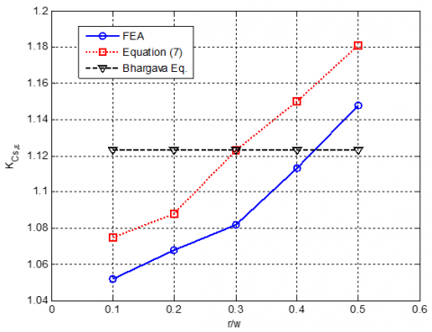
In this equation, the values of i=1.8, j=0.1 and k=1.5 means that the effect of r⁄w and t/r in these equation terms is non-linear. Also, the values of d1=0.28 and d2=0.1 indicate that the effect of the interaction effect of t/r and Cs⁄t has a positive effect of the value of KCs,ϵ. The comparison between the results of KCs,ϵ of Eq. (7), KCs,ϵ from [10], and the present FEA is depicted in Figure 5. For this figure, Cs⁄t=0.25 and t⁄r=1.
Figure 5. Comparison between Eq. (7), Bhargava's Eq. and FEA for KCs,ϵ
Apparently, the KCs,ϵ obtained from the equation [34] is independent from r/w. In contradiction, Eq. (7) and FEA results proves a proportional relationship between KCs,ϵ and r/w which further justifies the selection of Eq. (6) form.
4.4 The Kθc,ϵ equation
The general form of Kθc,ϵ equation is selected to be similar to that developed by Bhargava and Shivakumar [34], as:
$K_{\theta c, \epsilon}=1+m\left(\theta_{c}-100^{\circ}\right)$ (8)
where, m is the slope and it is a function of Cs/t and t/r, thus:
$m=A_{1}\left(\frac{t}{r}\right)^{\lambda}$ (9)
$A_{1}=\frac{C_{s}}{t}\left[-0.003+0.078\left(\frac{C_{s}}{t}\right)-0.078\left(\frac{C_{s}}{t}\right)^{2}\right]$ (10)
$\lambda=\frac{C_{S}}{t}\left[3.6-9.6\left(\frac{C_{S}}{t}\right)+7.8\left(\frac{C_{s}}{t}\right)^{2}\right]$ (11)
In the equations above, Kθc,ϵ equals to 1 when θc=100° and the slope m reduces to zero for Cs/t=0 or for a straight shank configuration. The selection of the equation models in Eq. (8) to Eq. (12) was based on the findings [22, 34] in which the slope (m) of Eq. (8) was found to be a function of both Cs/t and t⁄r therefore Eqns. (9), (10) and (11) were introduced.
Although Eq. (8) to Eq. (11) are expressed as presented by [34], the coefficients of Eq. (10) and Eq. (11) are obtained based on the present FEA data and are different from those [34]. The results of the present Kθc,ϵ equation are validated with the present FEA results and Kθc,ϵ equation in the study [34], as presented in Figure 6. In this figure, r⁄w=0.1, t⁄r=2 and Cs/t=0.3. From this figure, the results of the present equation of $K_{\theta c, \epsilon}$ compares well with FEA and literature.
Figure 6. Comparison between Eq. (8), Bhargava's Eq. and FEA for Kθc,ϵ
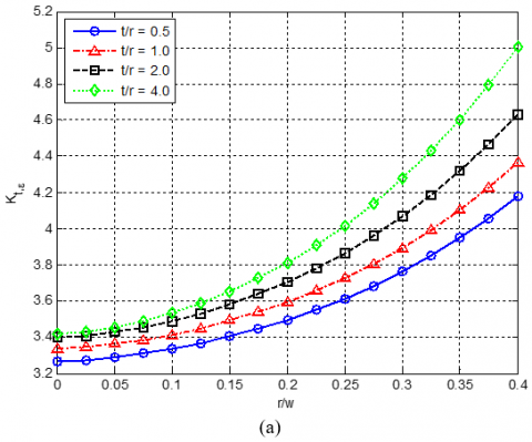
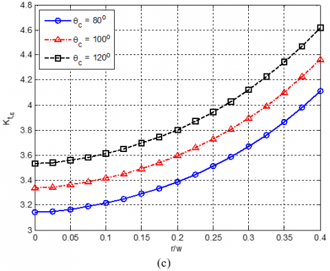
The effect of the dimensionless geometric parameters r/w, t/r, Cs/t and θc as well as Poisson’s ratio on Kt,ϵ value using the presently developed and verified equation are presented in this section. Specifically, Figure 7 introduces the effect of the radius to width ratio (r/w). Apparently, the Kt,ϵ value increases as r/w increases. In other words, as the plate becomes narrower, and the plate edge gets closer to the hole radius. Besides, these three figures show that $K_{t, \epsilon}$ value gets higher as t/r, Cs/t and θc increase.
Figure 7. Effect of r/w on Kt.ϵ at different (a) t⁄r, (b) Cs⁄t and (c) θc values (ν=0.3)
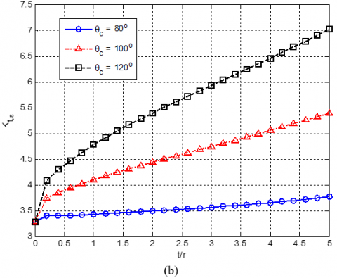
Similarly, Figure 8 shows the effect of t/r at different Cs⁄t and θc values. As shown in Figure 8(a), for small countersink depths (Cs⁄t=0.1), the plate thickness to radius ratio t/r effect is minor. However, for larger countersink depths (Cs⁄t≥0.2), t/r effect becomes more significant. Also, as presented in Figure 8(b), the plate thickness effect becomes more effective for higher countersink angle systems. This could be explained as for higher countersink depths, the tapered surface of the hole will become thicker and therefore, extra force lines will be reoriented towards the straight shank portion of the countersunk hole.
Figure 8. Effect of t/r on Kt.ϵ at different (a) Cs⁄t and (b) θc values (ν=0.3)
Figure 9 represents the relationship between Kt.ϵ and Cs⁄t at different countersink angles. From this figure, generally, as Cs⁄t increases, the maximum SɛCF increases, too. Additionally, this effect becomes more effective for plates with higher countersinking angles.
Figure 9. Effect of Cs⁄t on Kt.ϵ (r/w=0.25, t/r=2 and ν=0.3)
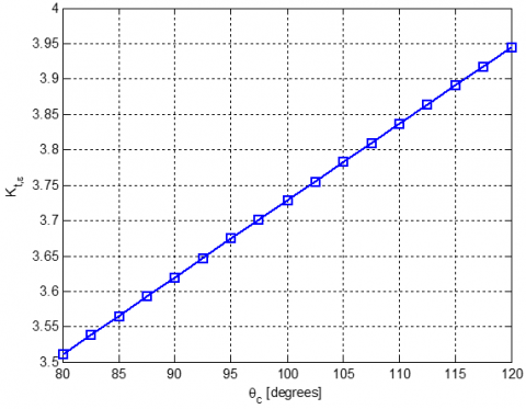
Figure 10 depicts the relationship between θc and Kt.ϵ. It is clearly seen that Kt.ϵ proportionally increases as θc increases. This is due to the fact that for larger countersink openings (larger θc) the hole further deviates from the straight shank configuration which results in higher values of SɛCF.
Figure 10. Effect of θc on Kt.ϵ (r/w=0.25, t/r=1, Cs⁄t=0.25 and ν=0.3)
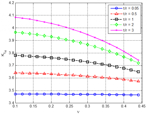
The effect of Poisson’s ratio (ν) effect on Kt.ϵ is presented in Figure 11. This figure shows that Poisson’s ratio effect varies from no effect, for thin plates (t/r=0.05), to significant effect, for thick plates (t/r=4). It also shows that the Kt.ϵ decreases as v increases.
Figure 11. Effect of ν on Kt.ϵ (r/w=0.25, Cs⁄t=0.25 and θc=100°)
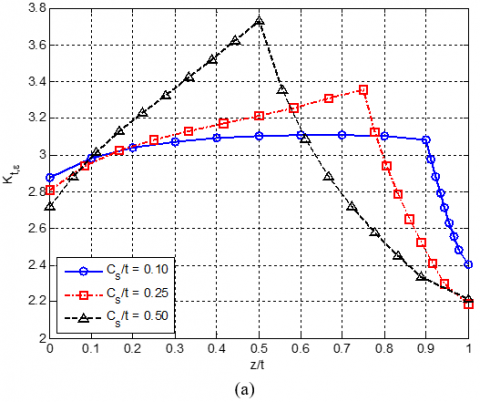
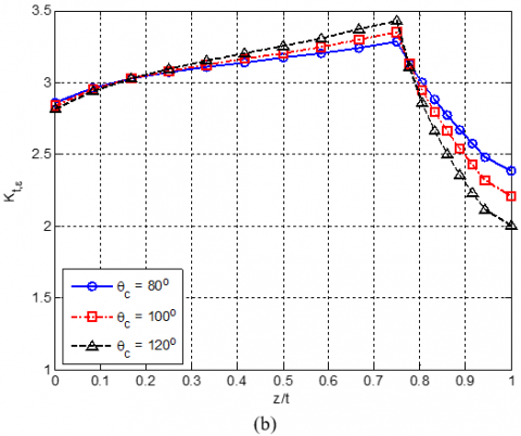
Finite element solutions were used to investigate the strain concentration factor distribution over the thickness of the countersunk hole. It was found that the maximum strain concentration factor value occurs at the side of the hole at 90 degrees from the load application direction. Figure 12 represents the strain concentration factor values variation over the thickness of the countersunk hole for different countersink depths and angles. From Figure 12(a), the location of the maximum strain concentration factor value changes with varying the countersink depth (Cs⁄t) value. On the other hand, the location of the maximum strain concentration factor value is kept fixed for different countersink angle (θc) values, as shown in Figure 12(b).
Appendix A lists the results of Kt.ϵ from the present FEA model, the newly developed equation in this study and the equation presented by Bhargava et al. for wide ranges of r/w, t/r and Cs⁄t at θc=100° and ν=0.3. The FEA data in table were for geometric configurations that were used in the fitting process and for new configurations that were generated for comparison and validation purposes. The relative error in Kt.ϵ of both empirical equations was calculated with respect to the present FEA data and appended in Appendix A as well. As it can be concluded from the error columns of this table, that for Cs⁄t <0.5 the error values in both equations are relatively small and comparable with each other.
Figure 12. Strain concentration factor variation over the thickness of the hole for different countersink (a) depths, and (b) angles (r/w=0.1, t/r=1, Cs⁄t=0.25 and ν=0.3)
Hence, no further significance of one equation over the other. However, for Cs⁄t≥0.5 the presently developed equation of Kt.ϵ is in better agreement with FEA data than that for Bhargava et al. equation, especially for higher r/w values and for most t/r ratios. This could be explained as the earlier equation of the SɛCF developed by Bhargava and Shivakumar [34], the KCs,ϵ equation was expressed in the terms of t/r and Cs⁄t only and did not consider the significant effect of r/w. In contrast, the present work suggests that KCs,ϵ is to include the effect of r/w of Eq. (6). Therefore, higher accuracy of the present equation is observed. Additionally, the negative error values in Bhargava et al. (2008) equation mean that this equation underestimates the Kt.ϵ values which could lead to erroneous results if it was used in an engineering design process. This further appraises the present Kt.ϵ equation over the old equation in Ref. [34].
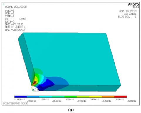
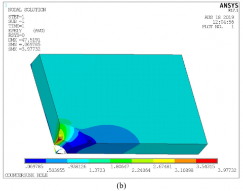
Figure 13 shows the stress and strain contour plots of a plate with a countersunk hole with r⁄w=0.1, t⁄r=2, Cs⁄t=0.5, θc=100° and ν=0.3. This figure shows that both stress and strain concentrations are located at the countersink hole edge, as mentioned previously. Also, this figure shows that the stress and strain distribution far from the whole are equal to E and 1, respectively, which are both equal to the nominal stress and strain values. Therefore, the stress and strain concentration factors could be easily calculated as 4.1 and 3.977, respectively.
Figure 13. (a) Stress and (b) strain contour plots
6.1 Conclusions
This paper presented an extensive three-dimensional finite element analysis for the strain concentration in countersunk holes subjected to uniaxial tension. The influence of the four non-dimensional geometric parameters: countersink angle (θc), thickness to radius ratio (t/r), countersink depth to plate thickness ratio (Cs/t) and radius to width ratio (r/w) and Poisson’s ratio (ν) on the strain concentration factor was investigated. Finite element analysis results showed that the maximum strain concentration is located at the countersinking edge of the hole and that is perpendicular to the load direction. Non-linear regression techniques were employed to develop an empirical equation for the strain concentration factor considering the limiting conditions and based of finite element data. The results of the equation were thoroughly correlated with finite element analysis results. Additionally, the present equation was compared to a previously developed equation by [34] and showed better agreement with FEA results especially for countersunk holes with high radius to width ratios.
6.2 Method limitations
The presently developed equation is accurate, simple, and easy to implement. However, it includes some limitations, thus, improvements are recommended. Firstly, the FEA data that was used to fit the equation were based on the assumption that the plate deformations are restricted to the linear and elastic range only. Nonetheless, in reality stress and strain concentration lead to high deformation regions which might change the case to a nonlinear problem. Thus, the results of this equation may not be very accurate for high concentration values, i.e., larger than 4. Secondly, the present work neglects the triaxiality of the stress and/or strain. Therefore, another study, which counts for the triaxiality of stress, is essential. Such work is available in the study of Tlilan et al. [36]. Lastly, the results of the current equation are highly recommended to be validated with experimental data for high-confident in the empirical formulations and findings.
The author wishes to deeply thank the Hashemite University for providing the necessary tools for this work.
|
b |
straight shank thickness |
|
$C_{s}$ |
countersink depth |
|
$E, v$ |
Modulus of Elasticity and Poisson’s ratio |
|
$K_{H}$ |
dimensionless factor, introduces the effect of the plate width on Kt,ϵ |
|
$K_{s s, \epsilon}$ |
dimensionless factor, introduces the effect of the plate thickness on Kt,ϵ |
|
$K_{C s, \epsilon}$ |
dimensionless factor, introduces the effect of the countersunk depth on Kt,ϵ |
|
$K_{t, \epsilon}$ |
theoretical strain concentration factor |
|
$K_{\theta c, \epsilon}$ |
dimensionless factor, introduces the effect of the countersink angle on Kt,ϵ |
|
h |
plate half-length |
|
r |
straight shank radius |
|
SCF |
stress concentration factor |
|
SɛCF |
strain concentration factor |
|
SS |
straight shank |
|
t |
plate thickness |
|
w |
plate half-width |
|
x, y, z |
Cartesian coordinate system |
|
$\theta_{c}$ |
countersink angle |
Appendix A. Comparison between FEA and current equation
|
r/w |
Cs/t=0.1 |
||||||||||||||
|
t/r=1 |
t/r=2 |
t/r=4 |
|||||||||||||
|
FEA |
Eq. (2) |
%E |
Bhargava et al. |
%E |
FEA |
Eq. (2) |
%E |
Bhargava et al. |
%E |
FEA |
Eq. (2) |
%E |
Bhargava et al. |
%E |
|
|
0.1 |
3.18 |
3.31 |
4.0 |
3.29 |
3.5 |
3.20 |
3.38 |
5.6 |
3.40 |
6.3 |
3.37 |
3.383 |
0.5 |
3.51 |
4.1 |
|
0.2 |
3.30 |
3.47 |
5.1 |
3.41 |
3.5 |
3.36 |
3.50 |
4.2 |
3.57 |
4.7 |
3.53 |
3.582 |
1.5 |
3.63 |
2.9 |
|
0.3 |
3.51 |
3.70 |
5.3 |
3.64 |
3.5 |
3.59 |
3.64 |
1.7 |
3.75 |
4.8 |
3.82 |
3.914 |
2.5 |
3.87 |
1.3 |
|
0.4 |
3.92 |
4.13 |
5.4 |
4.01 |
2.3 |
3.97 |
4.10 |
2.9 |
4.14 |
4.2 |
4.32 |
4.433 |
2.6 |
4.27 |
-1.2 |
|
r/w |
Cs/t=0.25 |
||||||||||||||
|
t/r=1 |
t/r=2 |
t/r=4 |
|||||||||||||
|
FEA |
Eq. (2) |
%E |
Bhargava et al. |
%E |
FEA |
Eq. (2) |
%E |
Bhargava et al. |
%E |
FEA |
Eq. (2) |
%E |
Bhargava et al. |
%E |
|
|
0.1 |
3.43 |
3.47 |
1.0 |
3.47 |
1.0 |
3.60 |
3.59 |
0.0 |
3.70 |
0.1 |
3.82 |
3.71 |
-3.0 |
3.99 |
4.4 |
|
0.2 |
3.57 |
3.65 |
2.4 |
3.59 |
0.7 |
3.76 |
3.81 |
1.5 |
3.80 |
1.2 |
4.04 |
4.00 |
-1.1 |
4.06 |
0.4 |
|
0.3 |
3.85 |
3.96 |
2.8 |
3.83 |
-0.5 |
4.09 |
4.18 |
2.2 |
4.05 |
-1.0 |
4.53 |
4.49 |
-0.9 |
4.33 |
-4.9 |
|
0.4 |
4.33 |
4.43 |
2.4 |
4.22 |
-2.5 |
4.68 |
4.76 |
1.8 |
4.47 |
-4.4 |
5.43 |
5.25 |
-4.6 |
4.78 |
-9.0 |
|
r/w |
Cs/t=0.5 |
||||||||||||||
|
t/r=1 |
t/r=2 |
t/r=4 |
|||||||||||||
|
FEA |
Eq. (2) |
%E |
Bhargava et al. |
%E |
FEA |
Eq. (2) |
%E |
Bhargava et al. |
%E |
FEA |
Eq. (2) |
%E |
Bhargava et al. |
%E |
|
|
0.1 |
3.81 |
3.77 |
-1.2 |
3.73 |
-2.3 |
4.03 |
4.03 |
0.0 |
4.08 |
1.2 |
4.37 |
4.50 |
3.1 |
4.57 |
4.7 |
|
0.2 |
3.99 |
4.00 |
0.3 |
3.86 |
-3.3 |
3.36 |
4.34 |
-0.4 |
4.23 |
-3.0 |
4.93 |
4.96 |
0.6 |
4.73 |
-4.0 |
|
0.3 |
4.36 |
4.38 |
0.5 |
4.11 |
-5.8 |
4.87 |
4.86 |
-0.3 |
4.51 |
-7.5 |
- |
- |
- |
- |
- |
|
0.4 |
5.03 |
4.97 |
-1.1 |
4.54 |
-9.7 |
5.99 |
5.76 |
-3.7 |
4.97 |
-17.0 |
- |
- |
- |
- |
- |
|
r/w |
Cs/t=0.75 |
||||||||||||||
|
t/r=1 |
t/r=2 |
t/r=4 |
|||||||||||||
|
FEA |
Eq. (2) |
%E |
Bhargava et al. |
%E |
FEA |
Eq. (2) |
%E |
Bhargava et al. |
%E |
FEA |
Eq. (2) |
%E |
Bhargava et al. |
%E |
|
|
0.1 |
4.05 |
4.10 |
1.4 |
3.94 |
-3.0 |
4.51 |
4.59 |
1.9 |
4.45 |
-1.4 |
- |
- |
- |
- |
- |
|
0.2 |
4.25 |
4.38 |
3.1 |
4.08 |
-4.0 |
4.80 |
4.99 |
4.0 |
4.60 |
-4.2 |
- |
- |
- |
- |
- |
|
0.3 |
4.70 |
4.84 |
3.1 |
4.35 |
-7.3 |
5.41 |
5.66 |
4.5 |
4.91 |
-9.5 |
- |
- |
- |
- |
- |
|
0.4 |
5.48 |
5.56 |
1.4 |
4.80 |
-12.4 |
- |
- |
- |
- |
- |
- |
- |
- |
- |
- |
[1] Boresi, A.P., Schmidt, R.J., Sidebottom, O.M. (1985). Advanced Mechanics of Materials (Vol. 6). New York: Wiley.
[2] Dowling, N.E. (2012). Mechanical behaviour of materials: Engineering methods for deformation, fracture, and fatigue. Pearson.
[3] Pilkey, W.D., Pilkey, D.F., Bi, Z. (2020). Peterson's Stress Concentration Factors. John Wiley & Sons.
[4] Savin, G.N. Stress concentration around holes. Pergamon.
[5] Shivakumar, K.N., Newman Jr, J.C. (1992). Stress concentrations for straight-shank and countersunk holes in plates subjected to tension, bending, and pin loading (Vol. 3192). National Aeronautics and Space Administration, Office of Management, Scientific and Technical Information Program.
[6] Shivakumar, K.N., Newman Jr, J.C. (1995). Stress concentration equations for straight-shank and countersunk holes in plates. Transactions-American Society of Mechanical Engineers Journal of Applied Mechanics, 62: 248-248. http://dx.doi.org/10.1115/1.2895916
[7] Wu, H.C., Mu, B. (2003). On stress concentrations for isotropic/orthotropic plates and cylinders with a circular hole. Composites Part B: Engineering, 34(2): 127-134. http://dx.doi.org/10.1016/S1359-8368(02)00097-5
[8] Kotousov, A., Lazzarin, P., Berto, F., Harding, S. (2010). Effect of the thickness on elastic deformation and quasi-brittle fracture of plate components. Engineering Fracture Mechanics, 77(11): 1665-1681. http://dx.doi.org/10.1016/j.engfracmech.2010.04.008
[9] Kotousov, A., Wang, C.H. (2002). Three-dimensional stress constraint in an elastic plate with a notch. International Journal of Solids and Structures, 39(16): 4311-4326. http://dx.doi.org/10.1016/S0020-7683(02)00340-2
[10] Li, Z., Guo, W., Kuang, Z. (2000). Three-dimensional elastic stress fields near notches in finite thickness plates. International Journal of Solids and Structures, 37(51): 7617-7632. http://dx.doi.org/10.1016/S0020-7683(99)00311-X
[11] Berto, F., Lazzarin, P., Wang, C.H. (2004). Three-dimensional linear elastic distributions of stress and strain energy density ahead of V-shaped notches in plates of arbitrary thickness. International Journal of Fracture, 127(3): 265-282. https://doi.org/10.1023/B:FRAC.0036846.23180.4d
[12] She, C., Guo, W. (2007). Three-dimensional stress concentrations at elliptic holes in elastic isotropic plates subjected to tensile stress. International Journal of Fatigue, 29(2): 330-335. https://doi.org/10.1016/j.ijfatigue.2006.03.012
[13] Enab, T.A. (2014). Stress concentration analysis in functionally graded plates with elliptic holes under biaxial loadings. Ain Shams Engineering Journal, 5(3): 839-850. https://doi.org/10.1016/j.asej.2014.03.002
[14] Kumar, A., Agrawal, A., Ghadai, R., Kalita, K. (2016). Analysis of stress concentration in orthotropic laminates. Procedia Technology, 23: 156-162. https://doi.org/10.1016/j.protcy.2016.03.012
[15] Jadvani, N., Dhiraj, V.S., Joshi, S., Kalita, K. (2017). Non-dimensional stress analysis of orthotropic laminates. Materials Focus, 6(1): 63-71. https://doi.org/10.1166/mat.2017.1377
[16] Zhou, Y., Fei, Q. (2017). Evaluation of opening-hole shapes for rivet connection of a composite plate. Proceedings of the Institution of Mechanical Engineers, Part C: Journal of Mechanical Engineering Science, 231(20): 3810-3817. https://doi.org/10.1177/0954406216652169
[17] Whaley, R.E. (1965). Stress-concentration factors for countersunk holes. Experimental Mechanics, 5(8): 257-261. https://doi.org/10.1007/BF02327149
[18] Cheng, Y.F. (1978). Stress-concentration factors for a countersunk hole in a flat bar in tension and transverse bending. Journal of Applied Mechanics, 45(4): 929-932. https://doi.org/10.1115/1.3424443
[19] Shivakumar, K.N., Bhargava, A., Hamoush, S. (2007). A general equation for stress concentration in countersunk holes. Cmc-Tech Science Press, 6(2): 71.
[20] Shivakumar, K.N., Bhargava, A., Newman Jr, J.C. (2007). A tensile stress concentration equation for countersunk holes. Journal of Aircraft, 44(1): 194-200.
[21] Bhargava, A., Shivakumar, K.N. (2007). Three-dimensional tensile stress concentration in countersunk rivet holes. The Aeronautical Journal, 111(1126): 777-786. https://doi.org/10.2514/1.22900
[22] Darwish, F., Gharaibeh, M., Tashtoush, G. (2012). A modified equation for the stress concentration factor in countersunk holes. European Journal of Mechanics-A/Solids, 36: 94-103. https://doi.org/10.1016/j.euromechsol.2012.02.014
[23] Darwish, F., Tashtoush, G., Gharaibeh, M. (2013). Stress concentration analysis for countersunk rivet holes in orthotropic plates. European Journal of Mechanics-A/Solids, 37: 69-78. https://doi.org/10.1016/j.euromechsol.2012.04.006
[24] Gharaibeh, M.A., Tlilan, H., Gharaibeh, B.M. (2021). Stress concentration factor analysis of countersunk holes using finite element analysis and response surface methodology. Australian Journal of Mechanical Engineering, 19(1): 30-38.
[25] Chaudhuri, J., Kalman, Z.H., Weng, G.J., Weissmann, S. (1982). Determination of the strain concentration factors around holes and inclusions in crystals by X-ray topography. Journal of Applied Crystallography, 15(4): 423-429. https://doi.org/10.1107/S0021889882012308
[26] Pandita, S.D., Nishiyabu, K., Verpoest, I. (2003). Strain concentrations in woven fabric composites with holes. Composite Structures, 59(3): 361-368. https://doi.org/10.1016/S0263-8223(02)00242-8
[27] Yang, Z., Kim, C.B., Cho, C., Beom, H.G. (2008). The concentration of stress and strain in finite thickness elastic plate containing a circular hole. International journal of Solids and Structures, 45(3-4): 713-731. https://doi.org/10.1016/j.ijsolstr.2007.08.030
[28] Ray-Chaudhuri, S., Chawla, K. (2018). Stress and strain concentration factors in orthotropic composites with hole under uniaxial tension. Curved and Layered Structures, 5(1): 213-231. https://doi.org/10.1515/cls-2018-0016
[29] Ball, D.L., Martinez, M., Baldassarre, A., Dubowski, D. M., Carlson, S.S. (2020). Analytical and Experimental Investigation of Elastic–Plastic Strain Distributions at 2-D Notches. Journal of Testing and Evaluation, 49(5). https://www.astm.org/jte20190924.html
[30] Zhu, S.P., Xu, S., Hao, M.F., Liao, D., Wang, Q. (2019). Stress-strain calculation and fatigue life assessment of V-shaped notches of turbine disk alloys. Engineering Failure Analysis, 106: 104187. https://doi.org/10.1016/j.engfailanal.2019.104187
[31] Guo, W., Guo, W.L. (2019). Formulization of three-dimensional stress and strain fields at elliptical holes in finite thickness plates. Acta Mechanica Solida Sinica, 32(4): 393-430. https://doi.org/10.1007/s10338-019-00091-w
[32] Tlilan, H.M., Jawarneh, A.M., Jawarneh, A., Tarawneh, M., Rababah, M., Smadi, O.A. (2019). Srain-concentration factor of internally pressurized thick-walled cylinders. International Journal of Applied Mechanics and Engineering, 24(1): 143-159. http://dx.doi.org/10.2478/ijame-2019-0010
[33] Hayajneh, M., Darwish, F.H., Alshyyab, A. (2014). A modelling strategy and strain concentration analysis for a countersunk hole in an orthotropic plate. International Journal of Design Engineering, 5(3): 175-192. http://dx.doi.org/10.1504/IJDE.2014.062354
[34] Bhargava, A., Shivakumar, K.N. (2008). A three-dimensional strain concentration equation for countersunk holes. The Journal of Strain Analysis for Engineering Design, 43(2): 75-85. https://doi.org/10.1243%2F03093247JSA334
[35] Heywood, R.B. (1952). Designing by photoelasticity. First edition, Chapman & Hall.
[36] Tlilan, H. M., Sakai, N., Majima, T. (2006). Effect of notch depth on strain-concentration factor of rectangular bars with a single-edge notch under pure bending. International Journal of Solids and Structures, 43(3-4): 459-474. https://doi.org/10.1016/j.ijsolstr.2005.03.069