Finite Element Modeling of Partially Composite Light-Gage Steel Tube Beam with Lightweight Concrete Deck Slab

A composite beam is composed of a steel beam and reinforced concrete. Composite beams provide greater economy and increase functionality. In order to have concrete slab and steel beam work together to resist bending under gravity loads, the slippage between them should be prevented by shear connectors [1].

Initially, these composite constructions were built using solid concrete slabs and steel beams. For casting solid concrete slabs, the use of temporary formwork is necessary, which is a time-consuming method; nevertheless, the invention of metal deck has eliminated the need for this formwork because the deck is set down on the steel beam before casting and linked to the beam using shear connectors to accomplish composite action [2].

A newer type of composite system was inserted into the building construction industry in the late twentieth century using light-gage cold-formed steel sections. Installation of light-gage steel floor beams does not necessitate the use of specialized crafts. Floor systems constructed on the framework of light-gage steel floor beams can be produced fast and accurately. However, the design of light-gage steel as non-composite members has necessitated the use of greater section sizes, demanding more research into their composite behavior [3]. This innovative composite system replaces the hot-rolled steel beam with a cold-formed steel beam to produce a lighter structure. This form of the composite system has been utilized in light industrial floor systems, and the low-rise residential building industries [4].

The design of shear connections is an important factor in composite beam design, the “Full” connection between the steel beam and the concrete slab means that there is no slide at the contact between the two parts. When a composite beam's shear connection is full, the bending strength of the beam is not increased by adding additional shear connectors [5].

In contrast, when fewer shear connectors are utilized than are required for a full shear connection, a steel beam with a concrete connection is referred to as "partial." The phrase "partial connection" does not relate to insufficient shear connections, but instead to a connection that produces an amount of slip that is non-negligible at the steel beam-concrete slab interface, affecting both the deformations and strength of the composite beam [5].

As full interaction is an ideal situation, because of the assumption of ideal rigid plastic assumption does not accomplish since all shear connectors are flexible to a certain level, full interaction is seldom accomplished in practice. Hence, partial interaction commonly appears in actual structures [6], and due to the limited space for the shear connectors when using a metal deck that is governs by its rib spacing partial interaction is used in this type of construction.

Since full-scale composite beam tests remain costly and time-consuming, FE modeling can be utilized to determine the ultimate load and the nonlinear response of such beams. Based on the validation procedure that has been published by the authors [7], which includes the calibrations parameters related to the partially composite cold-formed beam with lightweight concrete slab. This study aims to investigate the static behavior of partially composite light-gage cold-formed beam with lightweight concrete deck slab where in general this behavior is difficult to be estimated by the analytical methods.

3.1 Element type, surface contact, and boundary condition

A three-dimensional hexahedral element has been utilized to mimic the concrete and the headed stud connectors, While the shell element has been used for the light-gage steel beam and the metal deck. Also, a truss element has been used for the reinforcement.

2.png

Figure 2. Finite element model

For the contact between the concrete and the deck, as well as between the deck and the cold-formed beam surface-to-surface contact, has been imposed with friction constants equal to 0.5 and 0.01 respectively. An embedded technique has been utilized to link the shear stud and the concrete. Tie constraint has been used to link the shear stud with the cold-formed steel beam.

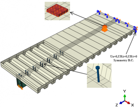
As shown in Figure 2, the finite element model for the proposed beam has been created by assuming symmetry at beam mid-span to simulate one-half of the composite beam in order to reduce the run time of the model.

Displacement controlled technique has been used to apply the load on the loading plates with enough time of loading to ensure the quasi-static condition using the dynamic explicit solver in ABAQUS. A comparison of the kinetic energy (KE) to the external work (EW) is presented in Figure 3. The figure shows that the kinetic energy is negligible, ensuring that a quasi-static condition is maintained.

3.png

Figure 3. Energy comparing

3.2 Material constitutive models

3.2.1 Concrete

The concrete has been assumed to be within the elastic range for the compression behavior up to stress of $0.4 f_{c}^{\prime}$ and tension behavior prior to cracking. Young's modulus, $E_{c}$, has been calculated according to ACI 318 relation. Poisson ratio, $v$, of $0.2$ has been used. After these stress levels, material constitutive models need to be defined.

There has been a great effort in recent years to create analytical models that correctly anticipate the plain concrete response to variable loading. Recently suggested models make use of general solid mechanics theories such as plasticity theory, and damage theory [8].

An initial yield surface, a hardening rule, and a flow rule were the three key assumptions that were utilized in the formulation of the theory of plasticity. Because the plasticity hypothesis was established for metals, adopting it to frictional materials such as concrete necessitates significant changes to these three assumptions [9].

The failure surface of the concrete is represented in Figure $4 \mathrm{a}$, which reflects the effect of the hydrostatic pressure. The deviatoric plane that perpendicular to the hydrostatic axis is presented in Figure $4 \mathrm{~b}$. The angle of similarity, $\theta$ is measured by projecting any axis onto the deviatoric plane and measuring it in both directions from 0 to 60 degrees. Tensile meridian is the meridian that corresponds to $\theta$ equals zero, and it is marked red. The compressive meridian is the meridian that corresponds to $\theta$ equals 60 , and it is marked blue [8,10].

Many models were suggested to represent the failure surface using plasticity theory, with models ranging from two parameters to the most complicated one with four parameters. The concrete damage plasticity model (CDP) was incorporated in ABAQUS. The CDP model has been used in a large number of FE analyses for concrete structures because of its fair performance and ease of use inside such a popular software program. The following describes the components of the CDP constitutive model.

4.png

Figure 4. Failure surface of concrete [10]

The CDP model utilizes the yield criterion established by Lubliner et al. [11] with the adjustment suggested by Lee and Fenves [12] considering the differences in strength evolution under compression and tension conditions.

The yield criterion proposed by Lubliner et al. [11] demands that the cohesion be stated clearly in the yield criterion as in Eq. (1) and relating the loss of strength to the vanishing of cohesion.

$F(\sigma)=\mathrm{c}$     (1)

where:

$F(\sigma)$ is a first-degree homogeneous function of stress components.

c is the cohesion.

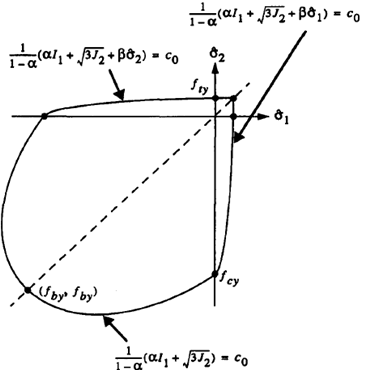
The yield criterion is expressed by Eq. (2), and it is represented in the plane space as in Figure 5:

5.png

Figure 5. The yield criterion in plane stress space [12]

$F(\sigma)=\frac{1}{1-\alpha}\left(\sqrt{3 J_{2}}+\alpha I_{1}+\beta\left\langle\hat{\sigma}_{\max }\right\rangle-\gamma\left\langle-\hat{\sigma}_{\max }\right\rangle=c\right.$       (2)

where:

$\alpha, \beta$ and $\gamma$ are dimensionless constant, $\hat{\sigma}_{\max }$ is algebraically maximum principal stress.

The yield criteria's algebraic formulation is notable in that they introduce the maximum principal stress term, $\beta\left\langle\hat{\sigma}_{\text {max }}\right\rangle$ or $\gamma\left\langle-\hat{\sigma}_{\max }\right\rangle$, its coefficient, $\beta$ or $\gamma$, is affected by the sign of $\hat{\sigma}_{\max }$ [13].

For stress conditions where tensile stress components are existing, i.e., $\hat{\sigma}_{\max }>0$, Eq. (2) becomes [13]:

$\frac{1}{1-\alpha}\left(\sqrt{3 J_{2}}+\alpha I_{1}+\beta\left\langle\hat{\sigma}_{\max }\right\rangle\right)=c_{0}$      (3)

For biaxial compression, i.e., $\hat{\sigma}_{\max }=0$, Eq. (2) becomes:

$\frac{1}{1-\alpha}\left(\sqrt{3 J_{2}}+\alpha I_{1}\right)=c_{0}$     (4)

For triaxial compression, i.e., $\hat{\sigma}_{\max }<0$, Eq. (2) becomes:

$\frac{1}{1-\alpha}\left(\sqrt{3 J_{2}}+\alpha I_{1}-\gamma\left\langle-\hat{\sigma}_{\max }\right\rangle\right)=c_{0}$     (5)

The parameter $\alpha$ can be calculated using Eq. (4) with assuming $c_{o}$ is equal to the initial uniaxial compressive, $f_{c y}$ $[12]$, and the equibiaxial compressive strength $f_{b y}$ state as:

$\alpha=\frac{\left(f_{b y} / f_{c y}\right)-1}{2\left(f_{b y} / f_{c y}\right)-1}$     (6)

Between $1.10$ and $1.16$, experimental values of $f_{b y} / f_{c y}$ are obtained, giving values of $\alpha$ between $0.09$ and $0.12$. ABAQUS default value for $f_{b y} / f_{c y}$ is $1.16$.

The parameter $\beta$ is calculated using Eq. (3) with $f_{c y}$ and the uniaxial tensile stress state, $f_{t y}$ as:

$\beta=\frac{f_{c y}}{f_{t y}}(\alpha-1)-(1+\alpha)$     (7)

Finally, the third parameter $\gamma$ only appears under states of triaxial compression, corresponding a stress state where $\hat{\sigma}_{\max }<0$. For the tensile meridians (T.M) $\left(\hat{\sigma}_{1}>\hat{\sigma}_{2}=\right.$ $\left.\hat{\sigma}_{3}\right):$

$\hat{\sigma}_{\max }=\frac{1}{3}\left(I_{1}+2 \sqrt{3 J_{2}}\right)$     (8)

While for the compressive meridians (C.M) $\left(\hat{\sigma}_{1}=\hat{\sigma}_{2}>\hat{\sigma}_{3}\right)$:

$\hat{\sigma}_{\max }=\frac{1}{3}\left(I_{1}+\sqrt{3 J_{2}}\right)$     (9)

With $\hat{\sigma}_{\max }<0$ the equations for the respective meridians are therefore [11]:

$(2 \gamma+3) \sqrt{3 J_{2}}+(\gamma+3 \alpha) I_{1}=(1-\alpha) f_{c y}$ T.M.

$(\gamma+3) \sqrt{3 J_{2}}+(\gamma+3 \alpha) I_{1}=(1-\alpha) f_{c y}$ C.M.       (10)

Hence, leading to the definition of the following parameter [11]:

$K_{C}=\frac{\left(\sqrt{J_{2}}\right)_{T . M .}}{\left(\sqrt{J_{2}}\right)_{C . M .}}$ at given $\mathrm{I}_{1}$     (11)

Then,

$K_{c}=\frac{\gamma+3}{2 \gamma+3}$     (12)

Thus, K_c is a dimensionless shape parameter, utilized to determine the form of the failure surface inside the deviatoric plane of Figure 4b. when K_c equals 1.0, the failure surface inside the deviatoric plane becomes a circle, which is consistent with the traditional Drucker-Prager hypothesis. According to Lubliner et al. [11] this value should range between 0.64 to 0.8 and the default value for ABAQUS is 2/3.

In the original model [11], isotropic hardening was used which gives good results in the monotonic loading but is not suitable for cyclic behavior of concrete. Because under the cyclic loading, the evolution of one strength (compression or tension) does not influence the evolution of the other strength.

As a result, the changes suggested by Lee and Fenves [12] incorporated a two variable hardening rule; one for controlling compression, $\tilde{\varepsilon}_{c}^{p l}$ and the other for controlling tension, $\tilde{\varepsilon}_{t}^{p l} . \mathrm{A}$ yield criterion with two variables is obtained by defining $(\beta)$, which is constant in Lubliner et al. yield criterion [11].

$\beta=\beta\left(\tilde{\varepsilon}^{p l}\right)$     (13)

$\beta=\frac{c_{c}\left(\tilde{\varepsilon}_{c}^{p l}\right)}{c_{t}\left(\tilde{\varepsilon}_{t}^{p l}\right)}(1-\alpha)-(1+\alpha)$     (14)

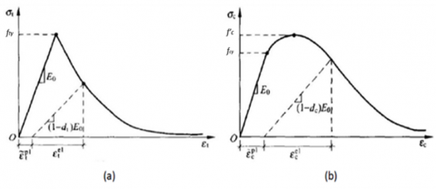
The nonlinear behavior of concrete is due to plasticity and damage processes. Microcracking, coalescence, and decohesion, among other things, can be ascribed to the damage process. Damage is often described by the degradation of stiffness. To characterize the damage, effective stress can be used [14]. The effective stress is defined as:

$\bar{\sigma}=E_{o}\left(\varepsilon-\varepsilon^{p l}\right)$     (15)

where:

E_o is the undamaged elastic stiffness that can be defined according to the theory of plasticity in which:

$\varepsilon^{e l}=\frac{\sigma}{E}$     (16)

Then, based on the previous equation the stress can be written as:

$\sigma=E\left(\varepsilon-\varepsilon^{p l}\right)$      (17)

By definition of the damage in stiffness degradation as scalar damage d that represented in Figure 6 then:

$E=(1-d) E_{o}$     (18)

Substituting Eq. (18) into Eq. (17) leads to the following relation:

$\sigma=(1-d) E_{o}\left(\varepsilon-\varepsilon_{p l}\right)$     (19)

6.png

Figure 6. Concrete response to uniaxial loading in tension (a), and compression (b) [15]

Or can be written using the effective stress as:

$\sigma=(1-d) \bar{\sigma}$     (20)

Then, the effective stress can be written as:

$\bar{\sigma}=\frac{\sigma}{1-d}$     (21)

Finally, the yield criteria using two hardening variables and in the effective stress space is written as:

$F\left(\bar{\sigma}, \tilde{\varepsilon}^{p l}\right)=\frac{1}{1-\alpha}\left(\sqrt{3 \bar{J}_{2}}+\alpha \bar{I}_{1}+\beta\left\langle\tilde{\varepsilon}^{p l}\right\rangle\left\langle\overline{\hat{\sigma}}_{\max }\right\rangle-\gamma\left\langle-\overline{\hat{\sigma}}_{\max }\right\rangle\right)=c_{c}\left(\tilde{\varepsilon}^{p l}\right)$     (22)

Because nonlinear volume change during hardening is a key property of concrete materials, the flow rule employed in the CDP model is the non-associated flow rule. The chose function for the CDP model is the hyperbolic formula of Drucker-Prager that represented by [15]:

$G=\sqrt{\left(e f_{t y} \tan \psi\right)^{2}+\bar{q}^{2}}-\bar{p} \tan \psi$     (23)

where:

e is the eccentricity, defines the rate over which the function approaches the asymptote,

ψ is the dilation angle;

f_ty is the uniaxial tensile stress at failure, extracted from the adopted tensile data.

In this study, the damage parameters have not been considered. The key parameters that have been introduced in ABAQUS are presented in Table 1.

Table 1. The defined parameters for the CDP model.

Compressive behavior. The model that has been used to mimic the uni-axial behavior of concrete was proposed by Yang et al. [16] according to Eq. (24). The uniaxial stress–strain curve that has been used to define the concrete compressive behavior is presented in Figure 7.

$\sigma_{c}=\left[\frac{\left(\beta_{1}+1\right)\left(\frac{\varepsilon_{c}}{\varepsilon_{o}}\right)}{\left(\frac{\varepsilon_{c}}{\varepsilon_{o}}\right)^{\beta_{1}+1}+\beta_{1}}\right] f_{c}^{\prime}$     (24)

where:

$\varepsilon_{o}=0.0016 \exp \left[240\left(f_{c}^{\prime} /_{E_{c}}\right)\right]$     (25)

$\beta_{1}=\left\{\begin{array}{c}0.2 \exp (0.73 \xi) \varepsilon_{c} \leq \varepsilon_{o} \\ 0.41 \exp (0.77 \xi) \varepsilon_{c}>\varepsilon_{o}\end{array}\right.$     (26)

Also,

$\xi=\left(\frac{f_{c}^{\prime}}{10}\right)^{0.67}\left(\frac{2300}{\omega_{c}}\right)^{1.17}$      (27)

ω_c is the concrete specimen’s density,

E_c is the Young’s modulus of concrete.

7.png

Figure 7. Stress-strain for concrete in compression

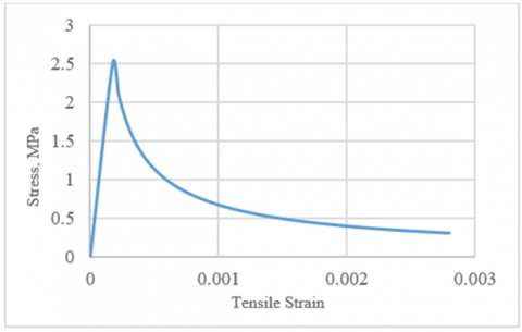
Tensile behavior. The concrete behavior in tension is defined in ABAQUS by means of the so called ‘tension stiffening’. The model that has been used in this study was proposed by Belarbi and Hsu [17]. The model is represented by the following equation:

$\sigma_{c t}=E_{c} \varepsilon_{c t} \varepsilon_{c t} \leq \varepsilon_{c r}$     (28)

$\sigma_{c t}=f_{t y}\left(\frac{\varepsilon_{c r}}{\varepsilon_{c t}}\right)^{0.4} \varepsilon_{c t}>\varepsilon_{c r}$     (29)

Modification is proposed for the previous formula as follow:

$\sigma_{c t}=f_{t y}\left(\frac{\varepsilon_{c r}}{\varepsilon_{c t}}\right)^{n}$     (30)

where:

n is the weakening function, in this analysis a value of 0.75 has been utilized [7],

ε_cr is the cracking concrete strain.

8.png

Figure 8. Stress-strain relation for concrete in tension

The uniaxial stress–strain curve that has been used to define concrete tensile behavior is presented in Figure 8, with $f_{t y}$, that has been calculated according to ACI 318 relation for modulus of rupture test.

3.2.2 Steel modeling

The cold-formed steel stress-strain behavior has been defined utilizing the model proposed by Gardner and Yun [18]. The model is defined using the following expression:

$\varepsilon=\left\{\begin{array}{c}\frac{\sigma}{E}+0.002\left(\frac{\sigma}{\sigma_{0.2}}\right)^{n}, \text { for } \sigma \leq \sigma_{0.2} \\ \frac{\sigma-\sigma_{0.2}}{E_{0.2}}+\left(\varepsilon_{u}-\varepsilon_{0.2}-\frac{\sigma_{u}-\sigma_{0.2}}{E_{0.2}}\right)\left(\frac{\sigma-\sigma_{0.2}}{\sigma_{u}-\sigma_{0.2}}\right)^{m} \\ +\varepsilon_{0.2}, \text { for } \sigma>\sigma_{0.2}\end{array}\right.$     (31)

where:

$E_{0.2}=\frac{E}{1+0.02 \mathrm{n} \frac{E}{f_{y}}}$     (32)

$\varepsilon_{u}=0.6\left(1-\frac{\sigma_{0.2}}{\sigma_{u}}\right)$     (33)

$\sigma_{u}=\left[1+\left(\frac{130}{\sigma_{0.2}}\right)^{1.4}\right] \sigma_{0.2}$     (34)

m and n are related to $\sigma_{0.05}$ or $\sigma_{0.1}$, and in the absence of experimental testing, values of 7.6 and 3.8 for m and n, respectively, can be used for flat coupons [18].

Elastic perfectly plastic model has been used in regards to the shear studs, and the steel reinforcement.

The deformed shape of the composite beam is presented in Figure 10, in addition to stresses of the light-gage beam at failure is shown in Figure 11. Stresses show that the beam is yielded where Mises stresses are larger than the uniaxial yield stress. This is due to strain hardening for the cold-formed steel beam.

Table 2 displays the results of the FE analysis, in addition to the design strength of the light-gage partially composite beams that have been calculated according to AISC [22].

Comparison of the results of Table 2 shows that the FE analysis is in agreement with the design strength according to AISC [22]. Because the standard of the light-gage cold-formed members, AISI [23] does not take into consideration the composite action, design according to AISC [22], is capable of computing the strength of this type of light-gage beam.

11.png

Figure 11. Stresses at the beam at failure

Table 2. Composite beams results.

5.1 Effect of concrete type and strength

As shown in Figure 12 changing the concrete type can have a minor effect on the stiffness and strength of the composite beam. Using normal weight concrete (NWC) increases the strength by 3.5%. This agrees with the results of Lasheen et al. [24], as they reported that results of experimental tests on composite beams revealed that changing the concrete type from NWC to LWC affected the ultimate load capacity by only 2.2%.

12.png

Figure 12. Effect of concrete type

Also, results of the analysis show that increasing the lightweight concrete compressive strength from 22.6 MPa to 50.5 MPa increases the capacity of the composite beam by 3% as presented in Figure 13.

13.png

Figure 13. Effect of lightweight concrete strength

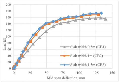
5.2 Effect of the slab width

The load-deflection curves of Figure 14 show that increasing the slab effective width from 500 to 1000 mm has a more significant influence on strength and stiffness than increasing the slab width from 1000 to 1500 mm. This is due to the effect of the shear lag phenomenon. Increasing the effective width from 500 to 1500 mm increases the strength of the light-gage composite beam by 9.87%.

14.png

Figure 14. Effect of the slab width

5.3 Effect of the thickness of the slab

15.png

Figure 15. Effect of the slab thickness

As shown in Figure 15, the thickness of the concrete slab affects the stiffness and strength of the partially composite light-gage lightweight concrete deck slab. Increasing the thickness of the slab from 150 mm to 200 mm increases the ultimate load of the system by 15.4%.

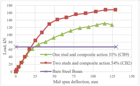
5.4 Effect of the degree of interaction

The effect of the degree of composite action on the behavior is presented in Figure 16. The figure also includes the strength of the bare light-gage beam for comparison purposes, which has been calculated according to AISI [23].

16.png

Figure 16. Effect of the composite action

The figure shows that employing partial interaction, even with a low degree of composite action, greatly enhances the strength. The composite action with a percentage of 31% only improves the strength of the beam by 95%. This improvement is increased by increasing the degree of interaction.

5.5 Effect of the yield stress of the beam

The load-deflection curves of partially composite light-gage beams with different yield stresses are presented in Figure 17. The yield stress of the cold-formed beam has a greater effect on the strength. Increasing the yield stress from 355 MPa to 700 MPa increases the strength by 38.5%.

17.png

Figure 17. Effect of the yield stress