Adedayo F. Adedotun* | Olanrewaju K. Onasanya | O. Olusegun Alfred | Olasumbo O. Agboola | Hillary I. Okagbue
© 2022 IIETA. This article is published by IIETA and is licensed under the CC BY 4.0 license (http://creativecommons.org/licenses/by/4.0/).
OPEN ACCESS
In the last five decades, Box Jenkins methodology has been in existence to model univariate time series data but fails or has limitations on modeling volatility. Most financial time series data do exhibit heavy tail and thick distribution, to this effect various parametric and semi-parametric non –linear time series models have been proposed two or three decades ago to capture volatility. However, this research entails measuring volatility and its forecasting using time series exchange rate annual data over the period from 1981 to 2020 (wide periodicity). The exchange rate was transformed to return, and parametric non –linear time series was modeled on it. It was found out that GARCH (1,2) reveals continuous volatility for short while and was the best model to predict the exchange rate volatility based on the evidence from measurement volatility tool; RMSE, MAE, MAPE among other extensions of GARCH models; EGARCH and TGARCH. EGARCH (1, 4) captures the asymmetry effect revealing that negative shocks will persistently have an effect on the volatility of the naira/dollar exchange rate.
returns, heteroscedasticity, volatility, non-linear time series, GARCH, exchange rate, autocorrelation
Time series is a wide area in statistics focusing on forecasting, and understanding the structural behaviors of series (stochastic random variable) [1]. Box Jenkins has dominantly analyzed time series data for forecasting in the last few decades and it is regarded with great usage by the scientific community. Also, structural models have been developed and applied in the last decades as well but were not able to outperform the originality of the random walk model proposed by Box and Jenkins in 1976 in aid of forecasting of the stochastic random variable [1, 2].
Forecasting techniques used in practice can be categorized into univariate time series models (GARCH) which capture volatility, and it has an edge above Box and Jenkins methodology of univariate time series models [3]. One of the limitations of the Box Jenkins method is that when there is the presence of threshold value, an exhibition of volatility clustering, the underlying structure of the series under study cannot be modeled but can be modeled with the idea of non-linear time series models.
Other types of forecasting techniques that have been in existence include but are not limited to market-based forecasting techniques. A recent development on forecasting time series or economic time series includes chaos theory and Artificial Neural Networks according to [4-6].
Hsieh [7] shows that different specifications of ARCH/GARCH models usually describe different currencies better than a unique model (STM or ARIMA models) because some currencies show a higher degree of seasonality than others due to higher amounts of export of goods around Christmas.
The multivariate regression approach has been used in many research to study and predict the exchange rate based on some listed variables but these have a limitation in the sense that macro-economic variables are available at most monthly periods precisely modeling of such explanatory variables will lead to a proportion change in the exchange rate [4, 8].
Majorly, applied econometricians use the giant statistical tool (least-squares model) as a natural choice to describe the nature of the exchange rate based on another macroeconomic variable listed above. The ARCH and GARCH models, which stand for autoregressive conditional heteroskedasticity and generalized autoregressive conditional heteroscedasticity respectively are designed to deal with just this issue [9].
In most recent times, they have been declared as a time series tool for capturing volatility or measuring volatility through the aid of measures of dispersion (variance or standard deviation) and these can be used in financial decisions concerning risk analysis, portfolio selecting, asset pricing and derivative pricing [10].
The volatility of financial assets has been a growing area of research. The traditional measure of volatility is represented by variance or standard deviation as stated above is unconditional and does not recognize the interesting patterns in asset volatility such as time-varying and cluster properties [11].
In Nigeria's context, two series were examined; structural adjustment program (SAP) where the exchange rate of Nigeria depreciated against the major intervention currency (US dollar) from 1970 to 1994). During this regime, investors and the capital market were not functioning very well. Some few business tycoons only invested in the capital market as a result of poor awareness. Also, decision-makers, business forecasters were not able to generate forecasts since the introduction of the regime. In 1994, the Nigerian government introduces foreign exchange markets (FEM) where little depreciation of naira was examined in 1994 and steady depreciation was examined in 1998 and 1999 and appreciated in 2005, 2006. A continuation of depreciation still exists to date. With this volatility in the exchange rate, little work has been done on modeling naira exchange rate volatility in Nigeria or how to capture the volatility using the GARCH models.
Recently, Musa et al. [12] makes use of GARCH models and the extension of GARCH models to model naira/dollar exchange using a short spine of periodicity. He found out that GJR – GARCH, and T- GARCH model shows the existence of a statistically significant asymmetric effect. But in this research work, the aim is to check for volatility measurement and its accuracy of predicting the naira exchange rate by applying a wide periodicity to check for the existence of leverage effect. The aim is attained by implementing extended GARCH families. The remainder of this research is section as section 2 focuses on data sources and empirical framework of ARCH models, section 3 describes the methodology, section 4 focuses on results and discussions, and section 5 describes the conclusion and possible recommendation for the research.
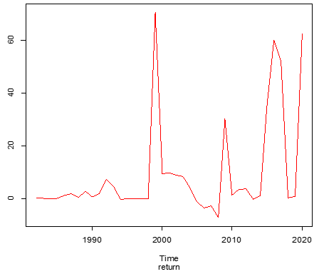
Figure 1. Graph of return series
Figure 2. Graph of exchange rate series
For volatility modeling, the data used in the present study consists of the annual foreign exchange rate of the naira/US dollar. The data was obtained from www.oanda.com with a sample period from 1981 to 2020. To model this data for volatility checking, different econometric time series models like ARMA, ARCH, GARCH, EGARCH, and TGARCH are critically employed. The exchange rate series obtained from www.oanda.com is therefore converted for the needs of fitting the model to a 1st difference as would be called “ $y_{t}$" return series, $x_{t}$ is the exchange rate series, then $y_{t}$ is called the return exchange rate and this is written as $y_{t}=x_{t}-x_{t-1}$. Figure 1 and Figure 2 shows the plot of the return series $y_{t}$ and the exchange rate series $x_{t}$.
This research work aims to identify volatility, measure volatility, and forecast using GARCH models and the selected extension of GARCH models via E- GARCH, and T- GARCH models using annual financial time series data which covers from 1981 to 2021 i.e., a widespread of data (exchange rate).
The E-GARCH model will capture the asymmetric effect of the response of disturbance on volatility while T – GARCH model will capture the leverage effect (the reaction of volatility to changes in exchange rate prices. This aim requires several steps to be taken, firstly a descriptive statistic is encouraged to be found to understand the nature of the exchange rate returns. It is expected that the mean return would be zero identifying stationarity else non-stationary.
It is also expectant that most financial data series have heavy tails i.e., their kurtosis exceeds 3 signifying that the distribution is leptokurtic and has a high value or peak; more also for normality the Jarque test will signify for the randomness of the return series i.e., are the data followed a normal distribution. It is also not to be forgotten the unconditional standard deviation which measures the spread of data values and the volatile measure, a high value of standard deviation signifies high volatility which reverse is the low volatility. Less, the asymmetric distribution (Skewness) which equals zero indicates normality, a negative value of Skewness indicates negative Skewness or left tail is particularly extreme while a positive value indicates positive Skewness or right tail is particularly extreme.
Once descriptive statistics are defined, we performed ADF test for test of stationarity of the return series. Once the unit root is tested, we developed a series of ARMA models of Eq. (1) below using least square estimation methods or a well-defined maximum likelihood estimation.
$\mu_{t}(\theta)=\varphi_{0}+\varphi_{1} y_{t-1}+\cdots+\varphi_{p} y_{t-p}+\theta_{1} \varepsilon_{t-1}+\cdots$
$+\theta_{q} \varepsilon_{t-q}+\epsilon_{t}$ (1)
where $\varphi_{0}=$ constant term, $\varphi_{1}, \ldots . \varphi_{p}=$ autoregressive coefficients from order 1 to $p^{t h}$ order and $\varepsilon_{1}, \ldots . \varepsilon_{q}=$ moving average coefficients from order 1 to $q^{t h}$ order and $\epsilon_{t}=$ ARMA error term.
According to Ref. [13], both methods of estimations give the same results. Akaike information and Bayesian information criteria are the two criteria used to select the best ARMA model, once the best ARMA model is developed we generate the error ($\varepsilon_{t}$) and check for the optimality of the best ARMA model, and plot the ACF (autocorrelation function) of the squared disturbance terms and also disturbance terms; if the disturbances hover the zero line, hence the best ARMA model is good. Once determine the optimality of the best ARMA model, we test for the ARCH effect (serial correlation in conditional variance).
Let
$\epsilon_{t}=y_{t}-\varphi_{0}-\sum_{i=1}^{p} \varphi_{i} y_{t-i}+\sum_{j=1}^{q} \theta_{j} \varepsilon_{t-j}$ (2)
Be the residuals of ARMA model of Eq. (1). The squared error series $\varepsilon_{i}^{2}$ is then check for conditional heteroscedasticity, which is known as the ARCH effect. The test for conditional heteroscedasticity is the Lagrange multiplier test of Engle [14]. The test is equivalent to usual F – statistics for testing $\alpha_{i}=0(i=1,2, \ldots \ldots q)$ in Eq. (3) below.
$\sigma_{t}^{2}=\alpha_{0}+\sum_{i=1}^{q} \alpha_{i} \varepsilon_{t-i}^{2}$ (3)
where $t=q+1, \ldots T$, where $\varepsilon_{t}$ denotes the error term, $q$ is the specified positive integer, and $T$ is the sample size. Specifically, the null hypothesis is:
$H_{0}: \alpha_{1}=\alpha_{2}=\ldots \ldots \alpha_{q}($ No Arch effect $)$
At least one parameter is not equal to zero (Arch effect). Let $S S R_{0}=\sum_{t=q+1}^{T}\left(\varepsilon_{t}^{2}-K\right)^{2}$, where $K=\frac{\sum_{t=q+1}^{T} \varepsilon^{2} t}{T}$, the sample is mean of $\varepsilon_{t}^{2}$ and let $S S R_{1}=\sum_{t=q+1}^{T} \hat{\varepsilon}_{t}^{2}$, where $\hat{\varepsilon}_{t}$, the least square residual of Eq (1) is, then we have:
$F_{s t a t}=\frac{\left(S S R_{1}-S S R_{2}\right) / q}{S S R_{1}(T-2 Q-1)} \sim X^{2}(q)$ (4)
where $q=$ the degree of freedom. The decision rule is to reject the null hypothesis if $F_{\text {stat }}>X^{2}{ }_{q}(\alpha)$ is the upper $100(1-$ $\alpha)^{t h}$ percentile of $X_{q}^{2}$ or the $\mathrm{p}$-value of $\mathrm{F}_{\text {stat }}$ is less than $\alpha$. Otherwise, no rejection of $\mathrm{H}_{0}$. if found ARCH effect is present i.e. a serial correlation in conditional variance of the error derived in Eq. (1), we estimate GARCH models to measure volatility. The essence of this ARCH effect will aid in the effect of exchange rate volatility which is been caused by some factors such as government policies or trade in balance etc. in fact this point out how effective are these factors have on naira dollar exchange rate.
3.1 Estimation techniques (arch models)
Three likelihood functions proposed by Fan and Yao [15] were used in ARCH estimation. If the series assumes normality, then, the likelihood function for the ARCH(q) model is:
$f\left(y_{1}, y_{2}, \ldots . y_{T} \mid \alpha\right)=f\left(y_{T} \mid \varphi_{t-1}\right) f\left(y_{T-1} \mid \varphi_{t-2}\right)$
$f\left(y_{q+1} \mid \varphi_{q}\right) f\left(y_{1}, y_{2}, \ldots \ldots y_{q} \mid \alpha\right)$ (5)
where $\alpha=\left(\alpha_{0}, \alpha_{1}, \ldots \ldots \alpha_{q}\right)^{\prime}$ and $f\left(y_{1}, y_{2} \ldots \ldots y_{q} \mid \alpha\right)$ is the joint probability density function of $y_{1}, y_{2}, \ldots y_{q}$,. Since the exact form of $f\left(y_{1}, y_{2} \ldots y_{q} \mid \alpha\right)$ is complicated, it is commonly dropped from the prior likelihood function, especially when the sample size is sufficiently large. This results in using the conditional likelihood function:
$f\left(y_{q+1}, y_{q+2} \ldots y_{T} \mid \alpha, y_{1}, y_{2}, \ldots . y_{q}\right)$ (6)
$=\prod_{t=q+1}^{T} \frac{1}{\sqrt{2 \pi} \sigma_{t}} e^{\left(\frac{-y^{2} t}{2 \sigma^{2} t}\right)}$
where, $\sigma_{t}^{2}$ can be evacuated recursively. We prefer the estimates obtained by maximizing likelihood estimates (MLE's) under which is easier to handle. In addition, it ensures that the maximum value of the log of the probability of Eq. (7) occurs at the same point as the original probability function in Eq. (5). Moreover, one of the usefulness of maximum likelihood estimate is that the population parameters in Eq. (5) are selected, by selecting the parameters such that the population distribution has the moments that are equivalent to the observed moments in the sample. Therefore, we can work with the simpler log-likelihood instead of the original likelihood. The conditional log likelihood function is:
$f\left(y_{q+1}, y_{q+2} \ldots y_{T} \mid \alpha, y_{1}, y_{2}, \ldots y_{q}\right)$
$=\sum_{T=q+1}^{T}\left(-\frac{1}{2} \ln (2 \Pi)-\frac{1}{2} \ln \left(\sigma_{t}\right)-\frac{1}{2} \frac{y_{t}^{2}}{\sigma_{t}^{2}}\right)$ (7)
Since the first two terms $\ln (2 \Pi)$ do not involve any parameter, the log likelihood function becomes:
$f\left(y_{q+1}, y_{q+2} \ldots y_{T} \mid \alpha, y_{1}, y_{2}, \ldots y_{q}\right)$
$=-\sum_{t=q+1}^{T}\left(\frac{1}{2} \ln \left(\sigma_{t}\right)+\frac{1}{2}\left(\frac{y_{t}^{2}}{\sigma^{2}}\right)\right)$ (8)
where, $\sigma_{t}^{2}=\alpha_{0}+\alpha_{1} \varepsilon_{t-1}^{2}+\alpha_{2} \varepsilon_{t-2}^{2}+\ldots \ldots \ldots \ldots \alpha_{q} \varepsilon_{t-q}$ can be evaluated recursively. Now in some applications, it is more appropriate to ensure that $\varepsilon_{t}$ follows a heavy tailed distribution such as standard t – distribution. There are two approaches to deal with the problem via robust inference and fat tail conditional distribution. For robust inference, see Ref. [16], for fat tailed conditional distribution; two approaches were involved parametric [17], non-parametric (semi parametric, [18], semi – non parametric density estimation; [19]. Following Ref. [17],
Let $X_{v}$ be a student $\mathrm{t}-$ distribution with $\mathrm{v}$ degrees of freedom. Then $v \operatorname{ar}\left(x_{v}\right)=\frac{v}{v-2}$ for $v>2$ and use $\varepsilon_{t}=\frac{x_{v}}{\sqrt{v(v-2)}}$, then probability density function of $\varepsilon_{t}$ is:
$f\left(\varepsilon_{t} \mid v\right)=\frac{\gamma\left(\frac{v+1}{2}\right)}{\gamma\left(\frac{v}{2}\right) \sqrt{(v-2) \Pi}}\left(1+\frac{\varepsilon_{t}^{2}}{v-2}\right)^{-\frac{v+1}{2}}$ $v>2$ (9)
where, $\gamma(x)$ is the use of gamma function i.e. $\gamma(x)=$ $\int_{0}^{\alpha} t^{x-1} e^{-t} \partial t$ now using $y_{t}=\varepsilon_{t} \sigma_{t}$ we obtain the conditional likelihood function of $y_{t}$ as:
$f\left(y_{q+1}, y_{q+2} \ldots y_{T} \mid \alpha, y_{1}, y_{2}, \ldots y_{q}\right)$$=\prod_{t=q+1}^{T} \frac{\gamma\left(\frac{v+1}{2}\right)}{\gamma\left(\frac{v}{2}\right) \sqrt{v-2} \pi} \frac{1}{\sigma_{t}}\left(1+\frac{y_{t}^{2}}{(v-2) \sigma_{t}^{2}}\right)^{-\frac{v+1}{2}}$$v>2$ (10)
Now we now refer to the estimates that maximize the prior likelihood function as the conditional MLE’s under the t – distribution. The degrees of freedom of the t – distribution can be specified a prior or estimated jointly with other parameters. Now a value between 3 or 6 is often used if it is per specified, then the conditional log likelihood function is:
$\ln \left(y_{q+1}, y_{q+2} \ldots y_{T} \mid \alpha, y_{1}, y_{2}, \ldots y_{q}\right)$
$=-\sum_{t=q+1}^{T}\left[\frac{v+1}{2} \ln \left(1+\frac{y_{t}^{2}}{(v-2) \sigma_{t}^{2}}+\frac{1}{2} \ln \left(\sigma_{t}^{2}\right)\right)\right]$ (11)
Now finally, it may assume a generalized error distribution GED), a situation where errors (the difference between the expected value of Eq. (3) and the observed values) are not normally distributed, i.e. if it does not obey the rule of symmetry or asymptotical rule. The probability function: is defined as:
$f(v s)=\frac{\operatorname{vexp}\left(-\frac{1}{2}\left|\frac{S}{v}\right|^{v}\right)}{\lambda 2\left(1+\frac{1}{v}\right) \gamma\left(\frac{1}{v}\right)}$$-\alpha<x \leq \alpha ; 0<v<\alpha$ (12)
And $\lambda=\left[2\left(\frac{-2}{v}\right) \frac{\gamma\left(\frac{1}{v}\right)}{\gamma\left(\frac{3}{v}\right)}\right]^{\frac{1}{2}}$, this distribution reduces to Gaussian distribution if $v=2$, and it has heavy tail i.e. the distribution will have a high kurtosis value indicating high peak of outliers when $v<2$. But if $v>2$, the distribution diverges as a result of convolutions problems or gradient problems.
3.2 Estimation technique (GARCH models)
From Fan and Yao [15], the conditional normal GARCH process is:
$\left(y_{t} \mid \varphi_{t-1}\right) \sim N\left(u_{t}(\theta), \sigma_{t}^{2}\right)$ (13)
And their conditional density is:
$f\left(y_{t} \mid \varphi_{t-1}\right) ; \theta=\frac{1}{\sqrt{2 \pi}} \sigma^{2} e^{\left(-\frac{1}{2}\left(\frac{y_{t}-\mu_{t}(\theta)}{\sigma^{2} t}\right)\right)^{2}}$ (14)
Its prediction error decomposition is given by:
$f\left(y_{T}, y_{T-1}, \ldots y_{1} ; \theta\right)$
$=f\left(y_{T} \mid \varphi_{t-1}\right) \times f\left(y_{T-1} \mid \varphi_{t-2}\right) \times f\left(y_{1} \mid \varphi_{0}\right)$ (15)
The log likelihood function is given by:
$\log \left(y_{T}, y_{T-1}, \ldots y_{1} ; \theta\right)=\log f\left(y_{T}, y_{T-1}, \ldots y_{1} ; \theta\right)$
$=-\frac{T}{2} \log 2 \pi-\frac{1}{2} \sum_{i=1}^{T} \log \sigma_{t}^{2}-\frac{1}{2} \sum_{t=1}^{T}\left(y_{t}-\mu_{t}(\theta)\right)^{2}$ (16)
Looking at Eq. (16), there is a non – linear function θ, so according to [15], numerical optimization techniques would be applied to estimate the persistent parameters in Eq. (17) below:
$\begin{aligned} \sigma_{t}^{2} &=\alpha_{0}+\alpha_{1} \varepsilon_{t-1}^{2}+\alpha_{2} \varepsilon_{t-2}^{2}+\cdots \alpha_{p} \varepsilon_{t-p}^{2} \\ &+\beta_{1} \sigma_{t-1}^{2}+\beta_{2} \sigma_{t-2}^{2}+\cdots \beta_{q} \sigma_{t-q}^{2} \end{aligned}$ (17)
We fit different types of GARCH models using the numerical optimization techniques as described above to estimate significant parameters and the best GARCH model is selected base on the smallest AIC and BIC criteria. The optimality of the GARCH model selected passed through diagnosis testing (plot of ACF of the standardized squared errors terms generated to test for continuous arch effect and the ACF of the standardized residuals for normality. If the ACF hovers around the line then the GARCH model estimated is satisfied. Hence the sum of coefficients of ARCH lags with GARCH lags would be less than unity and the coefficients of GARCH LAGS must be greater than zero. All the parameters must be (statistically significant). We proceed to perform the presence of ARCH effect from the ACF of the standardized squared residual if found out no ARCH effect we base our interpretation on the persistent parameter $\left(\beta_{j}\right)$ in Eq. (17). Estimation of E – GARCH and T- GARCH are estimated and the optimality of the models are followed in the same way as for GARCH models. For E – GARCH models the parameters that measure the leverage effect must be less than zero for the positivity of the variance while for the T – GARCH model; the parameter that measures the leverage effect must be greater than zero for the positivity of conditional variance.
3.3 H-step ahead forecast of the conditional variance of the error
Detail on the forecast conditional variance of GARCH model to be estimated in this research is given by:
Recall from GARCH $(1,1)$
$\sigma_{t}^{2}=\alpha_{0}+\alpha_{1} \varepsilon_{t}^{2}+\beta \sigma_{t}^{2}$ (18)
1 - step Ahead prediction is given by:
$\left(\sigma^{2}{ }_{h+k} \mid t\right)=\alpha_{0}+\alpha_{1} \varepsilon^{2}+\beta \sigma_{t}^{2}$ (19)
$k=$ step Ahead prediction is given by:
$\left(\sigma_{h+k}^{2} \mid t\right)=\alpha_{0}+\alpha_{1} \varepsilon_{t+k-1}^{2}+\beta \sigma_{t+k-1}^{2}$ (20)
For the long run – predictions:
$\lim _{k \rightarrow \infty}\left(h_{t+k} \mid t\right)=\frac{\alpha_{0}}{1-\alpha-\beta}=\bar{\alpha}_{0}$ (21)
For higher order $G A R C H(p, q)$
$\sigma_{t}^{2}=\alpha_{0}+\alpha_{1} \sum_{i=1}^{p} \varepsilon_{t-i}^{2}+\beta \sum_{j=1}^{q} \sigma_{t-j}^{2}$ (22)
Taking conditional expectations and assuming that a sample size of T, and for the conveniences that parameters in the forecast function are known, a forecast function for the optimal h – step ahead forecast of the conditional variance is written as:
$E\left(\sigma_{t+k}^{2} \mid \varphi_{t}\right)=\alpha_{0}$
$+\sum_{i=1}^{p} \alpha_{i} E\left(\varepsilon^{2} t \pm i \mid \varphi_{T}\right)+\sum_{j=1}^{q} \beta_{j} E\left(h_{t+k-j} \mid \varphi_{t}\right)$ (23)
When $\psi_{t}$ is the other relevant information pertaining to the forecast of $\sigma^{2}{ }_{t} \cdot E\left(\varepsilon^{2}{ }_{t+i} \mid \psi_{t}\right)=E\left(\sigma^{2}{ }_{t+i} \mid \psi_{t}\right)$ For $i>0$, $E\left(\varepsilon^{2}{ }_{t+i} \mid \psi_{T}\right)=\sigma^{2}{ }_{t+i}$ for $i>1 . E\left(\sigma^{2}{ }_{t+i} \mid \psi_{t}\right)$ is computed recursively. Thus, obtaining one- head forecast of $\sigma^{2}{ }_{t}$ is giving by $E\left(\sigma^{2}{ }_{t+1} \mid \psi_{t}\right)=\alpha_{0}+\alpha_{1} \varepsilon^{2}{ }_{t}+\beta \sigma^{2}{ }_{t}$ which is equivalent to Eq. (20). The procedure is continued and the long run predictor is equivalent to Eq. (21). According to Ref. [20], He stated that for GARCH $(1,1)$, the two step forecast is a little closer to the long run average variance than one - step forecast. Ultimately, the long run prediction is the same for all time periods as long as $\alpha_{i}+\beta_{i}<1$. Engle [20] regards that it is called the unconditional variance, hence GARCH models are mean reverting and conditionally heteroscedasticity but have a constant unconditional variance.
For $K$ - period's returns (exchange return):
$\varphi_{t+k}(K)=e_{t+k}+e_{t+k-1}+\cdots e_{t+1}$ (24)
For $K$-period return variance:
$\begin{aligned} \operatorname{var}\left(e_{t+k}(K) \mid \varphi_{t}\right) & \sim\left(\sigma_{t+k}^{2} \mid t\right)+\left(\sigma_{t+k-1}^{2} \mid t\right) \\ &+\cdots\left(\sigma_{t+1}^{2} \mid t\right) \end{aligned}$ (25)
3.4 Volatility forecast comparison
Four different measurement forecast accuracy tools would be used to compare the very best conditional heteroscedasticity models that provide an accurate forecast of the conditional variance via root mean squares, mean absolute error, mean absolute percentage error, and the Theil inequality. The mathematical representations of the above forecast measurement tool are as follows:
Root mean square $=\sqrt{\frac{\sum_{i=1}^{N}\left(\widehat{\sigma}^{2} t^{\left.-\sigma_{t}\right)^{2}}\right.}{N}}$ (26)
Mean absolute error $=\frac{\sum_{i=1}^{N}\left|\left(\hat{\sigma}^{2} t^{-\sigma_{t}}\right)^{2}\right|}{N}$ (27)
Mean absolute percentage error $=\sum_{i=1}^{N} \frac{\left|\left(\hat{\sigma}^{2} t^{-\sigma_{t}}\right)^{2}\right|}{\sigma_{t}}$ (28)
Theil inequality $=\frac{R M S E}{\sqrt{\frac{\sum_{i=1}^{N} \hat{\sigma}^{2} t}{N}}+\sqrt{\frac{\sum_{i=1}^{N} \sigma^{2} t}{N}}}$ (29)
where N is the number of out sample observations, $\sigma_{t}$ is the actual volatility at forecasting period “t” measured as the squared daily return, and $\hat{\sigma}^{2} t$ is the forecast at volatility at “t”. The first measurement forecasting tool would be used to forecast for the same series across all different conditional heteroscedasticity models. The smallest error indicates the better forecasting ability of that model according to the criteria. Under the Theil inequality, it is expected that the coefficient or the value of Theil would be zero which would indicate a perfect fit. Theil lies between 0 and 1. It is of necessity to understand the variability between volatility forecast from the actual series and variability between the mean of volatility forecast from the actual mean series. The following proportions define both clearly.
Bias proportion $=\frac{\sum_{i=1}^{N}\left(\hat{\sigma}^{2} t-\bar{y}\right)^{2} /{ }_{N}}{\sum_{i=1}^{N}\left(\hat{\sigma}^{2} t^{\left.-\sigma_{t}\right)^{2}} /_{N}\right.}$ (30)
This measures how far the mean difference of the volatility is from the mean of the actual series. The absolute range of tolerance error between the mean difference of the volatility and that of the mean of the observed series should not exceed $\pm 1.5 \%$ and there is no need for normalization of this difference.
Variance proportion $=\frac{\left(\delta_{\hat{y}}-\delta_{y}\right)^{2}}{\sum_{i=1}^{N}\left(\hat{\sigma}^{2} t-\sigma_{t}\right)^{2} /_{N}}$ (31)
This measures the variance of the volatility forecast from the variation of the actual series. Where $\delta_{\hat{y}}, \delta_{y}$ are the biased standard deviation of $\hat{\sigma}_{t}$ and $\sigma_{t}$ respectively.
Covariance proportion $=\frac{2(1-r) \delta_{\hat{y}} \delta_{y}}{\frac{1}{N} \sum_{i=1}^{N}\left(\widehat{\sigma}_{t}-\sigma_{t}\right)}$ (32)
This measures the remaining unsymmetrical forecasting errors. It is expected to be close to unity so that all the bias would be concentrated on it and allow variance proportion and bias proportion to be small.
It is mandatory to check for normality of the exchange rate return series, the asymmetry distribution of the return, and the tail nature of the return. To this effect, Table 1 presents the descriptive statistics of the return. From Table 1 above, the mean of the return series is almost zero but still can be interpreted as the return is stationary and also it exhibits volatility clustering. This can be easily seen from Figure 1, wide swings of data points. In terms of volatility, the standard deviation is so high of value (1.34666) indicating high volatility i.e., continuous rise in changes of exchange rate series and widespread of data values.
Table 1. Descriptive statistics of return series (sample period 1981:2021)
|
Variable |
Mean |
Median |
Standard dev. |
Skewness |
Kurtosis |
Jarqua Bera |
P - value |
|
Return |
0.0187 |
0.000 |
1.34666 |
14.796 |
736.789 |
1.67E+8 |
0.000 |
Table 2. ADF unit root test on exchange returns
|
Variable |
lag |
Intercept |
Trend plus intercept |
||
|
Exchange rate return |
ADF stat |
Critical value |
ADF stat |
Critical value |
|
|
1 |
-72.932 |
-3.43 (1%) |
-72.937 |
-3.964 (1%) |
|
|
2 |
-59.140 |
-59.149 |
|||
|
3 |
-52.322 |
-2.863 (5%) -2.567 (10%) |
-52.333 |
-3.413 (5%) -3.128 (10%) |
|
|
4 |
-48.589 |
-48.604 |
|||
|
|
5 |
-43.075 |
-43.092 |
||
Existence of positive Skewness and non – asymmetric distribution presence (i.e., the right tail is particularly at the extreme. It is empirical that most financial series deviate from normality (mean zero). The kurtosis value indicates a high value which indicates tall and thick distribution (leptokurtic) distribution since the kurtosis value exceeds 3. Most financial time series data do have heavy tails. A rejection of normality was rejected by Jarqua Bera test since its $p-$ value $(0.00)$ was less than the exact probability value of 0.05 and 0.01 level of significance. Hence meaning that the exchange return is non-normal distributed. We proceed to test for stationarity of the exchange return using the procedures discussed by Dickey and Fuller [21]. Table 2 displays the ADF test of return using two assumptions in the test equations; intercept, trend plus intercept up to lag 5.
This test was based on ADF test and was conducted on the levels of the return. The full sample period is from 1981 to 2020 annual exchange rate data. For the test, five lags were chosen to study the stationarity of the return using two assumptions: intercept and trend plus intercept.
Based on the five lags chosen, the ADF test statistics for all the five lags were greater than ADF critical value at $1 \%, 5 \%$, and $10 \%$ respectively indicating that the return is stationary at level form up to five (5) lags. To proceed in modeling volatility, it is expected for the return to be stationary and has ADF test has confirmed it is stationary. We proceed to develop an ARMA model, we regress the return with a constant “c" and generate the errors or residual then series of ARMA models were developed. The best ARMA model was chosen base on $A I C$ and $B I C$, based on the criteria’s $A R M A(2,1)$ was found to be the best among the five ARMA models we built. Table 3 reports the summary of its component.
Table 3. ARMA (2, 1) model components
|
Variable |
Coefficients |
Std. Error |
T. stat. |
Prob. |
|
$\left(\phi_{1}\right)$ |
0.11066 |
0.5225 |
1.3501 |
0.177 |
|
$\left(\phi_{2}\right)$ |
-0.1168 |
0.0115 |
-10.137 |
0.000 |
|
$\operatorname{Res} 1\left(\theta_{1}\right)$ |
-1.2586 |
0.8227 |
-1.5298 |
0.01261 |
Res 1: denotes the 1st lagged period at time (t-1) of the residual.
The sample period covers from 1981 to 2020 with 41 observations after adjusting the endpoints. With attaining AIC of value 3.402 and BIC value of 3.405.
The optimality of the model ARMA (2, 1) was judged by the ACF of squared residual. Table 4 displays the value of ACF of squared residual up to lag 10.
Table 4. Autocorrelation function of squared residual of ARMA (2, 1) model
|
Lag |
ACF |
PACF |
Q-stat. |
P-value |
|
1 |
0.005 |
0.05 |
0.2083 |
0.648 |
|
2 |
0.001 |
0.001 |
0.2211 |
0.895 |
|
3 |
0.002 |
0.002 |
0.2564 |
0.968 |
|
4 |
0.002 |
0.002 |
0.2760 |
0.991 |
|
5 |
0.01 |
0.01 |
1.0076 |
0.962 |
|
6 |
0.003 |
0.003 |
1.0929 |
0.982 |
|
7 |
0.002 |
0.001 |
1.1106 |
0.993 |
|
8 |
0.001 |
0.001 |
1.1245 |
0.997 |
|
9 |
0.001 |
0.001 |
1.1334 |
0.999 |
|
10 |
0.002 |
0.002 |
1.614 |
0.999 |
From Table 4, the AFC values of the squared residual of $A R M A(2,1)$ model hover round the zero-line indicating that residuals are normally distributed or presence of no serial correlations. Since the error is Gaussian, hence $A R M A(2,1)$ is selected to be accurate. We proceed to test for ARCH effect, we generated the squared residual from the $A R M A(2,1)$ model estimated and modeled it in a linear combination to the past lagged terms of the squared residuals with the presence of constants. Following the usage of AIC and BIC criteria for selecting the model, it was found out that ARCH was selected. Table 5 presents the model component.
Table 5. ARCH (1) Model components
|
Variable |
Coefficient |
Std. error |
T. stat. |
P-value |
|
$\alpha_{0}$ |
1.80389 |
0.57098 |
3.15924 |
0.0016 |
|
$\operatorname{Res} 1(-1) \alpha_{1}$ |
0.005292 |
2.0116 |
4.45616 |
0.04483 |
Res 1(-1): squared residual lagged at (t-1) periods.
The sample period covers from 1981 to 2020 with 41 observations after adjusting the endpoints. With attaining $A I C$ of value $10.6297$ and $B I C$ value of $10.63156 .$
From Table 5 , the coefficient of the squared residual at lagged $(t-1)$ period was less than 1 and significant since its p-value $(0.04483)$ is less than $0.05$ level of significance. For testing hetereoskedasticity, the remaining components of $A R C H$ (1) are summarized below in Table $6 .$
From Table 6, it shows that F -stats indicated as (***) shows that it is great to reject the null hypothesis of (no arch effect) or no presence of conditional heteroscedasticity since the p-value to have a larger value of F- stat > 6.208 is 0.02648 lesser than exact probability value at 0.05. Hence, we conclude that ARCH (1) model shows the presence of conditional heteroscedasticity or error variance is serially correlated. The interpretation of the coefficient obtained signifies that volatility of the return in a current period (t) has little effect from the volatility exhibited in the past month.
We further justify studying the volatility persistence, by building the different GARCH models, and AIC and BIC criteria was been used to identify the best GARCH class model. Based on the AIC & BIC it was found out that GARCH (1, 2) model was found to be the best among series of higher GARCH orders. Table 7 reports the component of GARCH (1, 2) model.
The sample period covers from 1981 to 2020 with 41 observations after adjusting the endpoints. With attaining $A I C$ of value 3.338842 and BIC value of 3.34256.
The expectation for the sum of $\left(\alpha_{i}+\beta_{i}\right)$ was less than 1 i.e., 0.738455 measured the volatility of shocks today affects through the volatility of next periods. The entire primary non – negativity condition of both $A R C H$ and $G A R C H$ coefficients were significantly identified and all coefficients were statistically significant since their p-value was less than observed probability at $1 \%$ and $5 \%$. The persistent parameter $\left(\beta_{1}\right)$ and $\left(\beta_{2}\right)$ allows for continuous volatility of exchange returns since greater than zero. This is to say that the exchange rate will continue to exhibit wide swings for some periods and later be adjusted for short-term periods. This volatility will continue for 1 month from this current time till the next 5 months. The adequacy of GARCH $(1,2)$ model estimated was subjected to the correlogram of the squared residual generated from the model. Table 8 displays the correlogram value of the squared residuals from the estimated $G A R C H(1,2)$ up lags 10.
Table 6. Remaining components of $A R C H(1)$
|
$R^{2}$ |
0.000028 |
Mean Dependent |
1.8134 |
|
Adjusted $R^{2}$ |
-0.000107 |
S.D dependent |
49.1915 |
|
S.E of regress |
49.19418 |
AIC |
10.6297 |
|
Log likelihood |
-39503.27 |
BIC |
10.6315 |
|
Durbin Watson |
2.023 |
***F.stat. |
6.208 |
|
Sum of Sq. Res |
17983 |
***Pvalue of F. stat |
0.02648 |
Table 7. GARCH (1, 2) model estimates
|
Variable |
Coefficient |
Std. Error |
Z. stats |
P-value |
|
$\alpha_{0}$ |
0.562480 |
0.032578 |
17.2658 |
0.000 |
|
$\alpha_{1}$ |
0.077368 |
0.005285 |
14.6379 |
0.000 |
|
$\beta_{1}$ |
0.089273 |
0.015626 |
5.71327 |
0.000 |
|
$\beta_{2}$ |
0.571814 |
0.021569 |
26.5127 |
0.000 |
Table 8. Autocorrelation function of squared Residual of GARCH (1, 2) model
|
Lag |
ACF |
PACF |
Q-stat. |
Pvalue |
|
1 |
0.005 |
0.05 |
0.2131 |
0.644 |
|
2 |
0.001 |
0.001 |
0.2266 |
0.893 |
|
3 |
0.002 |
0.002 |
0.2631 |
0.907 |
|
4 |
0.002 |
0.002 |
0.2835 |
0.991 |
|
5 |
0.01 |
0.01 |
1.0295 |
0.96 |
|
6 |
0.003 |
0.003 |
1.1172 |
0.981 |
|
7 |
0.002 |
0.001 |
1.1356 |
0.992 |
|
8 |
0.001 |
0.001 |
1.1502 |
0.997 |
|
9 |
0.001 |
0.001 |
1.1595 |
0.999 |
|
10 |
0.002 |
0.002 |
1.1886 |
0.98 |
It can be observed that from lag 1 up to $\operatorname{lag} 15$, the $A C F$ values hover round the zero line, and also their $p$ - values are all greater than $1 \%$ and $5 \%$. This result indicates that there is no presence of serial correlation in error variance, and $G A R C H(1,2)$ model is well fit for return of this kind even after subjecting it to a high-frequency data. A further measure of asymmetric effect (positive and negative) on volatility was judge through the implementation of $E-G A R C H$ models and also measure of leverage effect i.e., the reaction of volatility to changes in return. Table 9 presents the summary coefficients of $A R M A(2,1), G A R C H(1,2)$ model and as well as $E-G A R C H$ and $T-G A R C H$ coefficients for comparisons.
Both estimations of $E-G A R C H$ and $T-G A R C H$ are estimated with Marquardt algorithm with maximum iteration at 200 . The $A R C H$-term was none. $E-G A R C H(1,4)$ and $T-G A R C H(1,2)$ were found to be the best model and statistically significant to measure the asymmetry effect of shocks on volatility and volatility changes in exchange return respectively. The value in parenthesis indicates $Z-$ stats. and $p$-value.
From Table 9 , it reports that the asymmetry parameter $\gamma=$ $-0.080297$ of $E-G A R C H(1,4)$ is less than zero i.e., satisfy the condition for asymmetry effect to take place and it is statistically significant and allows a negative shock will automatically have a high value in volatility. These negative shocks may arise from changes in government policies of Nigeria, structural instability of the foreign exchange market from the central bank of Nigeria, trade-in balancing, and other negative factors. While for $T-G A R C H$, the parameter which measures the leverage effect $\gamma=0.095578$ satisfies the condition for the presence of leverage effect. The leverage parameter is also statistically significant since its $p-$ value $(0.00)$ is less than the observed probability.
Table 9. Summary of coefficients of ARMA, ARCH, and GARCH
|
Coeff |
ARMA (2,1) |
ARCH (1) |
GARCH (1,2) |
E-GARCH (1,4) |
T-GARCH (1,2) |
|
\phi_{1} |
0.11066 |
- |
- |
- |
- |
|
\phi_{2} |
-0.1168 |
- |
- |
- |
- |
|
\theta_{1} |
-1.2586 |
- |
- |
- |
- |
|
\alpha_{0} |
- |
1.8038 |
0.56248 |
- |
- |
|
\alpha_{1} |
- |
0.00529 |
0.07737 |
-0.009491 |
-0.0003 |
|
$\beta_{1}$ |
- |
- |
0.08927 |
1.134361 |
0.337257 |
|
$\beta_{2}$ |
- |
- |
0.571814 |
0.001357 |
0.483613 |
|
$\beta_{3}$ |
- |
- |
- |
-0.522890 |
- |
|
$\beta_{4}$ |
- |
- |
- |
0.377235 |
- |
|
$\omega$ |
- |
- |
- |
0.008522 |
0.255566 |
|
$\gamma$ |
- |
- |
- |
-0.08029 (78.2959) (0.0000) |
0.095578 (14.1366) (0.000) |
Table 10. Autocorrelation function of squared Residual of EGARCH (1, 4) model
|
Lag |
ACF |
PACF |
Q-stat. |
P_value |
|
1 |
0.015 |
0.025 |
0.3231 |
0.724 |
|
2 |
0.0041 |
0.0131 |
0.4367 |
0.802 |
|
3 |
0.032 |
0.064 |
.342 |
0.802 |
|
4 |
0.102 |
0.022 |
0.1376 |
0.873 |
|
5 |
0.03 |
0.0167 |
2.0425 |
0.8843 |
|
6 |
0.003 |
0.0891 |
1.6243 |
0.892 |
|
7 |
0.602 |
0.301 |
1.1356 |
0.984 |
|
8 |
0.0801 |
0.079 |
1.8552 |
0.99 |
|
9 |
0.0901 |
0.067 |
1.3695 |
0.99 |
|
10 |
0.0120 |
0.093 |
1.3735 |
0.98 |
Table 11. Autocorrelation function of squared Residual of TGARCH (1, 2) model
|
Lag |
ACF |
PACF |
Q-stat. |
P_value |
|
1 |
0.205 |
0.2315 |
0.30183 |
0.555 |
|
2 |
0.256 |
0.0321 |
0.2378 |
0.901 |
|
3 |
0.1045 |
0.02054 |
0.241 |
0.8521 |
|
4 |
0.045 |
0.0321 |
0.2910 |
0.8892 |
|
5 |
0.091 |
0.01 |
1.178 |
0.971 |
|
6 |
0.0932 |
0.003 |
2.178 |
0.9432 |
|
7 |
0.0283 |
0.00298 |
3.162 |
0.8932 |
|
8 |
0.001 |
0.001 |
1.9273 |
0.991 |
|
9 |
0.001 |
0.0034 |
1.9126 |
0.999 |
|
10 |
0.0357 |
0.00218 |
1.72 |
0.991 |
The simple interpretation of the leverage parameter is that the higher volatility the more the changes in the exchange rate. This characterized that Nigeria exchange market will continue to experience high volatility of exchange rate and this will persistently to exhibit. Both $E-G A R C H(1,4)$ and $T-G A R C H$ were subjected to diagnostic testing, and it was found out that both correlograms of theirs squared errors hovers around the zero-line indicating that both models are a good fit. Tables 10 and 11 presents the value of the correlogram of $E-G A R C H$ and $T-G A R C H$.
We proceed ahead and compare the accuracy of volatility forecast among the series of extension GARCH models. Table 12 presents the summary of the comparison of the accuracy of volatility forecast.
Table 12. Comparison of the accuracy of volatility forecast among extension of GARCH models
|
Measurement Volatility error |
ARCH (1) |
GARCH (1,2) |
EGARCH (1,4) |
TGARCH (1,2) |
|
RMSE |
0.0898 |
0.054323 |
0.7045 |
0.06435 |
|
MAE |
0.0679 |
0.000431 |
0.04345 |
0.07645 |
|
MAPE |
71.4341 |
60.4594 |
78.4697 |
84.6431 |
|
Theil Inequality |
0.0081 |
0.04 |
0.1643 |
0.24578 |
|
Variance proportion |
0.000321 |
0.03478 |
0.05647 |
0.21045 |
|
Bias proportion |
0.004 |
0.03214 |
0.03247 |
0.07645 |
|
Covariance proportion |
0.80445 |
0.76453 |
0.87643 |
0.64324 |
From Table 12, it reports that $G A R C H(1,2)$ model was found to predict more accurately the conditional variance of the error, where its measurement tools were lower among the measurement tools of other extensions of GARCH models. This GARCH $(1,2)$ is also accurate in forecasting naira/dollar exchange rate volatility. Surprisingly its Theil inequality is close to zero and indicating that is a good fit to predict the naira/dollar exchange rate while reduction in bias in errors was close to zero in both biases, and variance proportion but both were accumulated in the covariance proportion. A little error of about 0.03214 was detected between the mean of the volatility and the mean of the actual return; likewise, also 0.03478 indicates little error between the variance of conditional variance forecast and variance of the return.
This paper focuses on the measurement of volatility and its forecasting evidence from the naira/dollar exchange rate using financial time series annual data from 1981 to 2020 with a total observation of 41 data points. The exchange rate was transformed to return by taking the first difference of exchange rate, the return was the dependent variable used to generate the result of this research. The return was subjected to a stationarity test and it was confirmed stationary at level form using ADF test. The return exhibited volatility clustering, $A R M A(2,1)$ was modeled on return, and the errors were generated. It was found out that $A R C H$ effect was present. Due to the result of ARCH effect further prove of volatility was judged by GARCH and it was found out that there is continuous volatility and these volatilities will range from 1 month beginning from this period till next 5 five months (based on the high frequency of data). The volatility of shocks today affects the volatility of the next 5 months. For asymmetry measurement, $E G A R C H(1,4)$ was the model that captured it and it reveals that negative shocks (change in government policies, restructure of foreign exchange market by the central bank of Nigeria) will persistently have effect in volatility of naira/dollar exchange rate. TGARCH captures leverage effect presence and confirms that the higher the volatility, the higher the changes in Nigeria exchange rate. This means that Nigeria's exchange rate will continue to exhibit volatility. For accuracy of volatility forecast, based on three measurement volatility tools it was confirmed that GARCH $(1,2)$ model was the best model to predict the conditional variance and other stylized facts.
According to [12], $T S-G A R C H$ model was able to fit the naira/dollar exchange rate and this model was attained base on a small sample period, but this research confirms a GARCH $(1,2)$ base on a high frequency of data points. According to [7], different specifications of $A R C H / G A R C H$ model usually describe different currencies better than a unique model. Hence, further research on higher GARCH family-like component GARCH and an asymmetric component could be investigated to study more on the asymmetry and persistent leverage effect.
The possible recommendation of this research emphasizes the central bank of Nigeria to maintain a proper structure of the foreign exchange market as this serves as a major factor that could linger higher in volatility and also increase in export system and perfection in trading system in other to avoid persistent volatility on exchange rate.
[1] Olatayo, T.O., Adedotun, A.F. (2014). On the test and estimation of fractional parameter in ARFIMA model: Bootstrap approach. Applied Mathematical Sciences, 8(96): 4783-4792. http://dx.doi.org/10.12988/ams.2014.46498
[2] Okagbue, H.I., Adamu, M.O., Iyase, S.A., Edeki, S. O., Opanuga, A.A., Ugwoke, P.O. (2015). On the uniqueness and non-commutative nature of coefficients of variables and interactions in hierarchical moderated multiple regression of masked survey data. Mediterranean Journal of Social Sciences, 6(4): 408-417. http://dx.doi.org/10.5901/mjss.2015.v6n4s3p408
[3] Moosa, I. (2001). Triangular arbitrage in the spot and forward foreign exchange markets. Quantitative Finance, 1(4): 387-390. https://doi.org/10.1080/713665833
[4] Adedotun, A.F., Taiwo, A.I., Olatayo, T.O. (2020). A reparametrised autoregressive model for modelling gross domestic product. Annals of the Faculty of Engineering Hunedoara, 18(2): 183-188.
[5] Okagbue, H.I., Adamu, M.O., Anake, T.A. Wusu A.S. (2019). Nature inspired quantile estimates of the Nakagami distribution. Telecommunication Systems, 72(4): 517-541. http://dx.doi.org/10.1007/s11235-019-00584-6
[6] Onasanya O.K, Olusegun A.O., Adedotun A.F., Odekina G.O. (2021). Forecasting of exchange rate in regime switching: Evidence from non-linear time series model. The International Journal of Engineering and Science (IJES), 10(09): 01-12. http://dx.doi.org/10.9790/1813-1009010112
[7] Hsieh, D. (1989). Testing for nonlinearity in daily foreign exchange rate changes. Journal of Business, 62(3): 339-368.
[8] Onasanya, O.K., Adeniji, O.E. (2013). Forecasting of exchange rate between Naira and US dollar using time domain model. International Journal of Development and Economic Sustainability, 1(1): 45-55.
[9] Osabuohien, E., Obiekwe, E., Urhie, E., Osabohien, R. (2018). Inflation rate, exchange rate volatility and exchange rate pass-through interactions: The Nigerian experience. Journal of Applied Economic Sciences, 2(56): 574-585.
[10] Adeyemi, O.A., Samuel, E. (2013). Exchange rate pass-through to consumer prices in Nigeria. European Scientific Journal, 9(25): 110-123.
[11] Longmore, R., Robinson, W. (2004). Modelling and forecasting exchange rate dynamics: An application of asymmetric volatility models. Bank of Jamaica, Working Paper, WP2004.
[12] Musa, Y., Tasi'u, M., Bello, A. (2014). Forecasting of Exchange Rate Volatility between Naira and US Dollar Using GARCH Models. International Journal of Academic Research in Business and Social Sciences, 4(7): 369-381. http://dx.doi.org/10.6007/IJARBSS/v4-i7/1029
[13] Kleiner, B. (1977). Time Series Analysis: Forecasting and Control. Technometrics, 19(3): 343-344.
[14] Engle, R.F. (1982). Autoregressive conditional heteroscedasticity with estimates of the variance of United Kingdom inflation. Econometrica: Journal of the Econometric Society, 50(4): 987-1007. https://doi.org/10.2307/1912773
[15] Fan, J., Yao, Q. (2008). Nonlinear time series: nonparametric and parametric methods. Springer Science & Business Media.
[16] Bollerslev, T., Wooldridge, J. M. (1992). Quasi-maximum likelihood estimation and inference in dynamic models with time-varying covariances. Econometric Reviews, 11(2): 143-172. https://doi.org/10.1080/07474939208800229
[17] Bollerslev. T. (1987). A conditional Hetereoskedasticity Time series model for speculative prices and rates of return. The Review of Economic and Statistics, 69(3): 542-547. https://doi.org/10.2307/1925546
[18] Engle, R.F., Gonzalez-Rivera, G. (1991). Semiparametric ARCH models. Journal of Business & Economic Statistics, 9(4): 345-359. https://doi.org/10.2307/1391236
[19] Gallant, A.R., Hsieh, D.A., Tauchen, G.E. (1991). On fitting a recalcitrant series: The pound/dollar exchange rate. Nonparametric and Semiparametric Methods in Econometrics and Statistics, Proceedings of the Fifth International Symposium in Economic Theory and Econometrics, pp. 199-240.
[20] Engle, R.F. (2001) GARCH 101: The use of ARCH/GARCH models in applied econometrics. Journal of Economic Perspectives, 15(4): 157-168. https://doi.org/10.1257/jep.15.4.157
[21] Dickey, D.A., Fuller, W.A. (1979). Distribution of the estimators for autoregressive time series with a unit root. Journal of the American Statistical Association, 74(366a): 427-431. https://doi.org/10.1080/01621459.1979.10482531