Mohamed A. Abdoon | Faeza Lafta Hasan*
© 2022 IIETA. This article is published by IIETA and is licensed under the CC BY 4.0 license (http://creativecommons.org/licenses/by/4.0/).
OPEN ACCESS
In this paper, we have introduced the analytical solutions of the Benjamin-Bona-Mahony equation and the (2+1) dimensional breaking soliton equations with the help of a new Algorithm of first integral method formula two (AFIM), by depending on mathematical software’s. New and more general variety of families of exact solutions have been represented by different structures of 3rd dimension plotting and contouring plotting with different parameters. So, the solution in this research is unique, new and more general. We can apply in computer sciences, mathematical physics, with a different vision, general and Programmable.
first integral method, Benjamin-Bona-Mahony equation, breaking soliton equation, symbolic computation
It has been previously observed that nonlinear evolution equations (NLEEs) play an important depicting of nonlinear phenomena. There are many domains regulated by studying of these equations such as fluid mechanics, plasma physics, hydrodynamics, elastic media and theory of turbulence, nonlinear optics, water waves, viscoelasticity, chaos theory, and different applications [1-5]. Several attempts have been made on these nonlinear equations which has taken a great deal, wide reputation and effective contribution in interpretation the same physical and engineering phenomena. The wave soliton pulse [6], a significant feature of nonlinearity, shows a perfect equilibrium between nonlinearity and dispersion effects. The first integral method is a powerful solution method was presented by the mathematician [7], where this method is characterized with its strength, with high accuracy and ease of application by relying on the characteristics and advantages of the differential equations as well as mathematical software in finding the exact traveling wave solutions for complex and nonlinear equations that specialized of nonlinear physical phenomena, so was applied to an important type of NLEEs and fractional equations as [8-11] with compare with other methods, for example the homotopy perturbation method [12], the generalized tanh method [13], homotopy analysis method [14], and several methods [15-22], the first integral method has proven its ability to solve various types of non-linear problems and distinguishes it from other methods by its applicable and the various solitary wave solutions that we obtain by using this method.
The general formula of NLPDEs is:
$w\left(F, F_{x}, F_{t}, F_{x x}, F_{x t}, \ldots \ldots \ldots\right)$ (1)
where, u(x,t) is the solution of (1) by using the wave transforms:
$f(x, t)=f(\zeta), \zeta=\alpha x-\beta t$ (2)
we get:
$\frac{\partial}{\partial t}(\cdot)=-\beta \frac{\partial}{\partial \zeta}(\cdot), \frac{\partial}{\partial x}(\cdot)=\alpha \frac{\partial}{\partial \zeta}(\cdot), \frac{\partial^{2}}{\partial t^{2}}(\cdot)$
$=\beta^{2} \frac{\partial^{2}}{\partial \zeta^{2}}(\cdot), \frac{\partial^{2}}{\partial x^{2}}(\cdot)$
$=\alpha^{2} \frac{\partial^{2}}{\partial \zeta^{2}}(\cdot)$ (3)
Then Eq. (1) transforms to the ODEs as:
$p\left(f, f^{\prime}, f^{\prime}, \ldots \ldots\right)=0$ (4)
A new independent variable:
$x(\zeta)=f(\zeta), y(\zeta)=f^{\prime}(\zeta)$ (5)
The system of ODE:
$x^{\prime}(\zeta)=y(\zeta) y^{\prime}(\zeta)=F(x(\zeta), y(\zeta))$ (6)
Because Eq. (6) represents autonomous system then, it is difficult to find the first integral for this system thus by depending on the qualitative theory of differential equation [23], we can obtain the general solution of this system directly. By applying the Division theory to option first integral Eq. (6), thus we will obtain the exact solution of Eq. (1), now let us recall the Division theory.
Theorem 2.1 [the division theorem] [6]
Assume that $\Phi(x, y)$ and $Q(x, y)$ are polynomials of two variables x and y in C [x, y] and $\Phi(x, y)$ is irreducible in C [x, y]. If $Q(x, y)$ vanishes at any zero point of $\Phi(x, y)$, then there exists a polynomial $H(x, y)$ in ℂ [X, Y] such that:
$Q(x, y)=\Phi(x, y) \mathrm{H}(x, y)$
We need to apply the (AFIM) on the form:
$u^{\prime \prime}(\zeta)-T\left(u(\zeta), u^{\prime}(\zeta)\right) u^{\prime}(\zeta)-R(u(\zeta))=0$ (7)
where, $T\left(u, u^{\prime}\right)$ is a polynomial in $u$ and $u^{\prime}$, and $R(u)$ is a polynomial with real coefficients?
Now choose $T\left(u, u^{\prime}\right)=0$, and $R(u)=A u^{2}+B u$, so Eq. (7) change, we get;
$u^{\prime \prime}(\zeta)-A u^{2}(\zeta)-B u(\zeta)=0$ (8)
Using Eq. (5) and Eq. (6), Eq. (8) is equivalent to the two-dimensional autonomous system;
$x^{\prime}(\zeta)=y(\zeta) y^{\prime}(\zeta)=A x^{2}(\zeta)+B x(\zeta)$ (9)
Now, we are applying the Division theorem to seek the first integral to Eq. (9), suppose that,
$x=x(\zeta)$ and $y=y(\zeta)$ are the nontrivial solution to Eq. (9) and;
$q(x, y)=\sum_{i=0}^{M} a_{i}(x) y^{i}=0$ which is an irreducible Polynomial in the complex domain $C[X, Y]$, thus:
$q[X(\zeta), Y(\zeta)]=\sum_{i=0}^{M} a_{i}(X(\zeta)) Y^{i}(\zeta)=0$ (10)
$a_{i}(X)(i=0,1,2, \ldots \ldots M$ are polynomial and $a_{M}(X) \neq 0$, Eq. (10) is called the first integral method. There exists a polynomial $g(X) X+h(X) Y$ in the complex domain $C[X, \mathrm{Y}]$ such that:
$q[X(\zeta), Y(\zeta)]=\sum_{i=0}^{M} a_{i}(X(\zeta)) Y^{i}(\zeta)=0$ (11)
We start our study by assuming m=1 in Eq. (11) gives;
$\sum_{i=0}^{1} a_{i}^{\prime}(X) Y^{i+1}+\sum_{i=0}^{1} i a_{i}(X) Y^{i-1}\left(A X^{2}+B X\right)$
$\quad=(g(x)+h(X) Y)\left(\sum_{i=0}^{1} a_{i}(X) Y^{i}\right)$ (12)
Equating the coefficients $Y^{i}(i=2,1,0)$ we have;
$a_{1}^{\prime}(X)=a_{1}(X) h(X)$ (13a)
$a_{0}^{\prime}(X)=a_{1}(X) g(X)+a_{0}(X) h(X)$ (13b)
$a_{1}(X)\left(A X^{2}+B X\right)=a_{0}(X) g(X)$ (13c)
From Eq. (13a), we conclude that $a_{1}(X)$ is a constant for easiness, we set $a_{1}(X)=1$, and $h(X)=0$. and equalize the degrees of $g(X), a_{1}(X)$ and $a_{0}(X)$, we deduce that degree $g(X)=1$ only, so assume that $g(X)=A_{0} X+B_{0}$, then we have $a_{0}(X)$ from Eq. (13b).
$a_{0}(X)=\frac{A_{0} X^{2}}{2}+B_{0} X+C_{0}$, (14)
where, $C_{0}$ is an arbitrary integration constant. Then we get a system of nonlinear algebraic equations by substituting $a_{1}(X), a 0(X)$ and $g(X)$ in Eq. (13c) and setting all the coefficients of powers X to be zero, when solve this system we have:
$\left\{A=0, B=0, A_{0}=0, B_{0}=0, C_{0}=C_{0}\right\}$,
$\left\{A=0, B=B_{0}^{2}, A_{0}=0, B_{0}=B_{0}, C_{0}=0\right\}$,
By the first set we get the travail solution, so neglected and we take only the second set of solutions and substituting in Eq. (10) we obtain:
$Y(\zeta)=\pm \sqrt{B} X(\zeta)$, (15)
Respectively. Combining equation Eq. (15) with Eq. (9), we have,
$X_{1}(\zeta)=C_{1} e^{\sqrt{B} \zeta}, X_{2} (\zeta)=C_{1} e^{-\sqrt{B} \zeta}$
$Y_{1}(\zeta)=\frac{C_{1}\left(\frac{1}{2} C_{1} A e^{2 \sqrt{B} \zeta}+B e^{\sqrt{B} \zeta} \right)}{\sqrt{B}}+C_{2}$ (16a)
$Y_{2}(\zeta)=-\frac{1}{2} \frac{C_{1}^{2} A e^{-2 \sqrt{B} \zeta}}{\sqrt{B}}-C_{1} \sqrt{B} e^{-\sqrt{B} \zeta}+C_{2}$ (16b)
Now when m=2 in Eq. (10), and $\mathrm{q}(\mathrm{X}, \mathrm{Y})=0$ this implies $\frac{\mathrm{dq}}{\mathrm{d} \xi}=0$,
$\sum_{i=0}^{2} a_{i}^{\prime}(X) Y^{i+1}+\sum_{i=0}^{2} i a_{i}(X) Y^{i-1}\left(A X^{2}+B X\right)$
$\quad=(g(x)+h(X) Y)\left(\sum_{i=0}^{2} a_{i}(X) Y^{i}\right)$ (17)
On equating the coefficients of $Y^{i}(i=3,2,1,0)$ on both sides of Eq. (17), we have,
$a_{2}^{\prime}(X)=a_{2}(X) h(X)$ (18a)
$q a_{1}^{\prime}(X)=a_{2}(X) g(X)+a_{1}(X) h(X)$ (18b)
$a_{0}^{\prime}(X)+2 a_{2}(X)\left(A X^{2}+B X\right) =a_{1}(X) g(X)+a_{0}(X) h(X)$ (18c)
$a_{1}(X)\left(A X^{2}+B X\right)=a_{0}(X) g(X)$ (18d)
From Eq. (18a), we conclude that $a_{2}(X)$ is a constant, $h(X)=0 .$ we set $a_{2}(X)=1$ for easiness, and equalize the degrees of $g(X), a_{1}(X)$ and $a 0(X)$, we deduce that degree $g(X)=1$ only, assume that $g(X)=A_{0} X+B_{0}$ then we find $a_{1}(X)$, and $a_{0}(X)$ from Eq. (18b) & Eq. (18c).
$a_{1}(X)=\frac{1}{2} A_{0} X^{2}+B_{0} X+C_{0}$, (19a)
where, $C_{0}$ is a constant integration.
$\begin{aligned} a_{0}(X)=\frac{1}{8} A_{0} X^{4} &+\frac{1}{2} A_{0} B_{0} X^{3}+\frac{1}{2} B_{0}^{2} X^{2} \\ &+\frac{1}{2} A_{0} C_{0} X^{2}+B_{0} C_{0} X-\frac{2}{3} A X^{3} \\ &-B X^{2}+D_{0} \end{aligned}$ (19b)
By choosing a constant integration $D_{0}$ to be zero and combining equation Eq. (19a) & Eq. (19b) with Eq. (18d), then we get a system of nonlinear algebraic equations when setting all the coefficients of powers x to be zero, and solve this system we obtain:
$\left\{A=0, B=\frac{1}{4} B_{0}^{2}, A_{0}=0, \quad B_{0}=B_{0}, C_{0}=0\right\}$, (20a)
$\left\{A=A, B=B, A_{0}=0, \quad B_{0}=0, C_{0}=0\right\}$, (20b)
$\left\{A=0, B=0, A_{0}=0, B_{0}=0, C_{0}=C_{0}\right\}$, (20c)
From (20a) we get solutions same as case m=1. While using Eq. (20b) in Eq. (10), we obtain:
$Y_{1}=\frac{1}{3} \sqrt{6 A X+9 B} X, \quad Y_{2}=-\frac{1}{3} \sqrt{6 A X+9 B} X$ (21)
Respectively, combining equation Eq. (21) with Eq. (9):
$X_{1}(\zeta)=X_{2}(\zeta)=\frac{3}{2} \frac{\mathrm{B}\left(\tanh \left(\frac{1}{2} \zeta \sqrt{B}+\frac{1}{2} C_{1} \sqrt{B}\right)^{2}-1\right)}{A}$ (22)
then
$Y(\zeta)=\frac{3}{2} \frac{\mathrm{B}^{3 / 2} \sinh \left(\frac{1}{2} \zeta \sqrt{B}+\frac{1}{2} C_{1} \sqrt{B}\right)}{A \cosh \left(\frac{1}{2} \zeta \sqrt{B}+\frac{1}{2} C_{1} \sqrt{B}\right)^{3}}+C_{2}$ (23)
When using Eq. (20c) in Eq. (10), and then Eq. (10) we obtain:
$X(\zeta)=-\zeta C_{0}+C_{1}$ (24)
$Y(\zeta)=\frac{1}{3} A \zeta^{3} C_{0}^{2}-A \zeta^{2} C_{1} C_{0}-\left(\frac{1}{2}\right) B \zeta^{2} C_{0}+A C_{1}^{2} \zeta+B C_{1} \zeta+C_{2}$ (25)
Eqns. (16a, b), (23) and (25) represent the general solutions for differential equations of the form Eq. (7).
Also known as the regularized long-wave equation (R=LWE) represent an appropriate model to study the dynamics of small-amplitude surface water waves propagating undirectional, while suffering non-linear and dispersive effects Many applications of (R=LWE) as ionacoustic waves in plasma, the undular bore as a result of the transverse long wave between a regular flow and static water, pressure waves in fluid-gas bubble mixtures, and phonon packets in nonlinear crystals. A generalized version is given by:
$u_{t}+a u_{x}+2 u u_{x}+b u_{x x t}=0$ (26)
We look for traveling wave solution in the form;
$u(x, t)=f(\zeta), \zeta=x-c t$ (27)
Substituting Eq. (27) into Eq. (26) gives:
$-c b f^{\prime \prime \prime}+2 f f^{\prime}+(a-c) f^{\prime}=0$ (28)
Integrating the Eq. (28) with respect to ζ and taking the integration constants to zero yields:
$f^{\prime \prime}-\frac{(a-c)}{b c} f-\frac{1}{b c} f^{2}=0$ (29)
Comparing Eq. (32) to formula (7), we get;
$A=\frac{1}{b c}, B=\frac{a-c}{b c}$ (30)
By substituting in Eqns. (16a, b), with Eq. (27) we get:
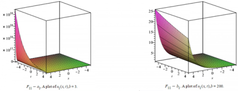
$u_{1}(x, t)=\frac{C_{1} \left(\frac{1}{2} C_{1} \frac{1}{b c} e^{2 \sqrt{\frac{a-c}{b c}(x-c t)}}+\frac{a-c}{b c} e^{\sqrt{\frac{a-c}{b c}(x-c t)}}\right)}{\sqrt{\frac{a-c}{b c}}}+C_{2}$ (31a)
$u_{2}(x, t)=-\frac{1}{2} \frac{C_{1}^{2} \frac{1}{b c} e^{-2 \sqrt{\frac{a-c}{b c}}(x-c t)}}{\sqrt{\frac{a-c}{b c}}}-C_{1} \sqrt{\frac{a-c}{b c}} e^{-\sqrt{\frac{a-c}{b c}}(x-c t)}+C_{2}$ (31b)
These solutions show that as Figures 1 and Figures 2 respectively.
From Eq. (23), with Eq. (27) the exact solution of Eq. (26) which represent as Figures 3 is:
$u_{3}(x, t)=\frac{3}{2} \frac{\mathrm{B}^{3 / 2} \sinh \left(\frac{1}{2} \zeta \sqrt{\frac{a-c}{b c}}+\frac{1}{2} C_{1} \sqrt{\frac{a-c}{b c}}\right)}{\frac{1}{b c} \cosh \left(\frac{1}{2} \zeta \sqrt{\frac{a-c}{b c}}+\frac{1}{2} C_{1} \sqrt{\frac{a-c}{b c}}\right)^{3}}+C_{2}$ (32)
From Eq. (25) we get:
$Y(\zeta)=\frac{1}{3 b c} \zeta^{3} C_{0}^{2}-\frac{1}{b c} \zeta^{2} C_{1} C_{0}-\left(\frac{1}{2}\right) \frac{a-c}{b c} \zeta^{2} C_{0}+\frac{1}{b c} C_{1}^{2} \zeta+\frac{a-c}{b c} C_{1} \zeta+C_{2}$ (33)
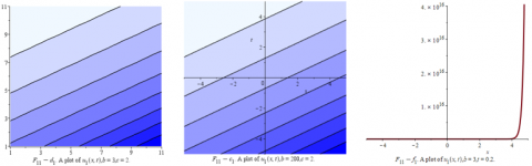
Figures 1. Eq. (31a) is illustrated in different plots with different dimensions in detail: the figure ($F_{11}-a_{1}$) is the 3-dimensional representation of (31a), the parametric values mentioned as $b=3, a=2.5, c=0.05, C_{1}=1, C_{2}=1 ;\left(F_{11}-b_{1}\right)$ is the representation of the 3-dimensional plotting of (31a) with same parametric value but $b=200 ;$ the plots $\left(F_{11}-c_{1}\right)$ and $\left(F_{11}-d_{1}\right)$ are representation of contour plotting of (31a) with same parametric values mentioned but $b=200, c=2$ and $b=3, c=2$ respectively, while $\left(F_{11}-f_{1}\right)$ here is the representation of the 2-dimensional plotting of Eq. (31a) with same parametric with $b=3, t=0.2$
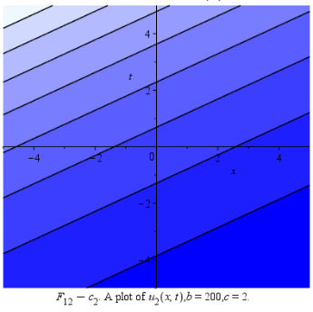
Figures 2. The physical representation of (31b) with different dimensions in detail: the figure ($F_{12}-a_{2}$) is the 3- dimensional representation of (31b), the parametric values mentioned as $b=3, a=2.5, c=0.05, C_{1}=1, C_{2}=1$, the graph $\left(F_{11}-b_{2}\right)$ is the representation of the 3-dimensional plotting of (31b) with same parametric value but $b=200,\left(F_{12}-c_{2}\right)$ is representation of contour plotting of (31b) with same parametric values mentioned and $=200, c=2$, while ($F_{11}-d_{2}$) here representation the 2-dimensional plotting of Eq. (31b) with same parametric with $t=0.2$
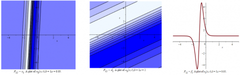
Figures 3. The illustration of Eq. (32) with different dimensions in detail: the figure ($F_{12}-a_{1}$) is the 3- dimensional representation of (32), the parametric values mentioned as $b=3, a=2.5, c=0.05, C_{1}=1, C_{2}=1$, here $\left(F_{12}-b_{1}\right)$ representation the 3- dimensional plotting of (32) with same parametric value but $=2 .$ The plots $\left(F_{12}-c_{1}\right),\left(F_{12}-d_{1}\right)$ are representation of contour plotting of (32) with same parametric values mentioned but different in $\left(F_{12}-d_{1}\right)$ where $c=2$, while $\left.F_{12}-f_{1}\right)$ here representation the 2- dimensional plotting of Eq. (32) with same parametric with $t=0.2$
Figures 4. The illustration of Eq. (34) with different dimensions in detail: the figure ($F_{12}-a_{2}$) is the 3- dimensional representation of (34), the parametric values mentioned as $b=3, a=2.5, c=0.05, C_{1}=1, C_{2}=1 ;$ here $\left(F_{12}-b_{2}\right)$ representation the 3- dimensional plotting of (34) with same parametric value but$b=200 ;$ the plot $\left(F_{12}-c_{2}\right)$ is representation of contour plotting of (34) with same parametric values mentioned but different in $b=200$ and $c=2 ;$ while $\left(F_{12}-d_{2}\right)$ here representation the 2- dimensional plotting of Eq. (34) with same parametric with $t=0.2$
By Eq. (27), the exact solution of Eq. (26) as form:
$\begin{aligned} u_{4}(x, t)=\frac{1}{3 b c}(&x-c t)^{3} C_{0}^{2} \\ &-\left(\frac{1}{b c} C_{1} C_{0}+\frac{a-c}{2 b c} C_{0}\right)(x\\ &-c t)^{2}+\frac{1}{b c} C_{1}^{2} \zeta \\ &+\frac{a-c}{b c} C_{1}(x-c t)^{2}+C_{2} \end{aligned}$ (34)
And this solution was shown in Figures 4.
This equation used to represent the Riemann wave along the y-axis with a long wave the x-axis which given by:
$\left\{\begin{array}{l}u_{t}-\alpha u_{x x y}+4 \alpha u v_{x}+4 \alpha u_{x} v=0 \\ u_{x}=v_{x}\end{array}\right.$ (35)
By looking for traveling wave solution in the form;
$u(x, y, t)=f(\zeta), \zeta=x+y-c t$ (36)
Integrating the second equation we get:
$u=v$ (37)
Substituting Eq. (37), into the first equation of the system gives:
$f^{\prime \prime}-\frac{c}{\alpha} f+3 f^{2}=0$ (38)
Comparing Eq. (38) to formula (7), we get:
$A=-3, B=\frac{c}{\alpha}$ (39)
By substituting in Eqns. (16a, b) we get:
$Y_{1}(\zeta)=\frac{C_{1}\left(\frac{-3}{2} C_{1} e^{2 \sqrt{\frac{c}{\alpha}}} \zeta+\frac{c}{\alpha} e^{\sqrt{\frac{c}{\alpha}} \zeta}\right)}{\sqrt{\frac{c}{\alpha}}}+C_{2}$ (40a)
$Y_{2}(\zeta)=\frac{3}{2} \frac{C_{1}^{2} e^{-2 \sqrt{\frac{c}{\alpha}}} \zeta}{\sqrt{\frac{c}{\alpha}}}-C_{1} \sqrt{\frac{c}{\alpha}} e^{-\sqrt{\frac{c}{\alpha}} \zeta}+C_{2}$ (40b)
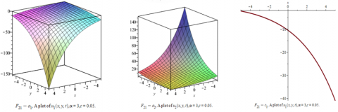
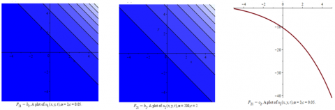
Figures 5. The illustration of (41a, b) with different dimensions in detail: the figures $\left(F_{21}-a_{1}\right)$ and $\left(F_{21}-a_{2}\right)$ are the 3- dimensional plotting representation of (41a) respectively) the parametric values mentioned as $\alpha=3, c=0.05, C_{1}=1, C_{2}=1 t=0.2 ;\left(F_{21}-b_{1}\right)$ and $\left(F_{21}-b_{2}\right)$ are the contour plotting representation of (41a, b) with same parametric value but $\alpha=3, c=0.05$ and $\alpha=200, c=2$ respectively; while $\left(F_{21}-c_{1}\right)$ and $\left(F_{21}-c_{2}\right)$ here representation the 2- dimensional plotting of (41a, b) with same parametric with $y=0.01$
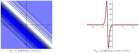
Figures 6. Every two figures $\left(F_{22}-a_{1}\right),\left(F_{22}-b_{1}\right)\left(F_{22}-a_{2}\right)$, and $\left(F_{22}-b_{2}\right)$ represent the Eq. (43) and Eq. (45) respectively with different dimensions and the parametric values mentioned as $\alpha=3, c=0.05, C_{1}=1, C_{2}=1 t=0.2$. only in $\left(F_{22}-b_{2}\right) \alpha=200, c=2 ;$ the figures $\left(F_{22}-c_{1}\right)$ and $\left(F_{22}-d_{1}\right)$ are are the contour plotting representation of Eq. (41) and Eq. (43) with parametric value$\alpha=200, c=2$ in first, $\alpha=3, c=2$ in second $\alpha=3, c=0.05$ in third figure; while $\left(F_{22}-f_{1}\right)$ and $\left(F_{22}-f_{2}\right)$ here representation the 2- dimensional plotting of Eq. (43) and Eq. (45) with same parametric with $y=0.01$
Then with Eq. (36) we have the exact solution (35) as:
$u_{1}(x, t)=\frac{\left(\frac{-3}{2} C_{1} e^{2 \sqrt{\frac{c}{\alpha}}(x+y-c t)}+\frac{C}{\alpha} e^{\sqrt{\frac{c}{\alpha}}(x+y-c t)}\right)}{\sqrt{\frac{c}{\alpha}}}+C_{2}$ (41a)
$\begin{aligned} u_{2}(x, t)=\frac{3}{2} \frac{C_{1}^{2} e^{-2 \sqrt{\frac{c}{\alpha}}(x+y-c t)}}{\sqrt{\frac{c}{\alpha}}} & \\ &-C_{1} \sqrt{\frac{c}{\alpha}} e^{-\sqrt{\frac{c}{\alpha}}(x+y-c t)}+C_{2} \end{aligned}$ (41b)
From Eq. (23),These solutions show that as Figures 5.
$Y(\zeta)=\frac{-1}{2} \frac{B^{3 / 2} \sinh \left(\frac{1}{2} \zeta \sqrt{\frac{c}{\alpha}}+\frac{1}{2} C_{1} \sqrt{\frac{c}{\alpha}}\right)}{\cosh \left(\frac{1}{2} \zeta \sqrt{\frac{c}{\alpha}}+\frac{1}{2} C_{1} \sqrt{\frac{c}{\alpha}}\right)^{3}}+C_{2}$, (42)
with Eq. (36) the exact solution of Eq. (26) as:
$u_{3}(x, t)$
$=\frac{-1}{2} \frac{B^{3 / 2} \sinh \left(\frac{1}{2}(x+y-c t) \sqrt{\frac{c}{\alpha}}+\frac{1}{2} C_{1} \sqrt{\frac{c}{\alpha}}\right)}{\cosh \left(\frac{1}{2}(x+y-c t) \sqrt{\frac{c}{\alpha}}+\frac{1}{2} C_{1} \sqrt{\frac{c}{\alpha}}\right)^{3}}+C_{2}$ (43)
From Eq. (25) we get:
$Y(\zeta)=-\zeta \quad C_{0}^{2}+3 \zeta^{2} C_{1} C_{0}-\frac{c}{2 \alpha} \zeta^{2} C_{0}$
$-3 C_{1}^{2} \zeta+\frac{c}{\alpha} C_{1} \zeta+C_{2}$ (44)
By Eq. (27), the exact solution of Eq. (35) as form:
$\begin{aligned} u_{4}(x, t)=-(x+&y-c t)^{3} C_{0}^{2} \\ &-\left(-3 C_{1} C_{0}\right.\\ &\left.+\frac{c}{\alpha} C_{0}\right)(x+y-c t)^{2} \\ &-3 C_{1}^{2}(x+y-c t) \\ &+\frac{c}{\alpha} C_{1}(x+y-c t)^{2}+C_{2} \end{aligned}$ (45)
These solutions show that as Figures 6.
In this section We give the illustration of our New Exact solutions in different dimensions. The graphs are shown for the (2+1) dimensional breaking soliton equations and the BBM equations by using Maple.
In this work we take the advantage of the characteristics of ordinary differential equations with first integral method which has many advantages because it is programmable.
Furthermore, we can apply the method to the nonlinear equation and fractional differential equation which can be reduced to the following form:
${u}''(\zeta )-T(u(\zeta ),{u}'(\zeta )){u}'(\zeta )-R(u(\zeta ))=0$
In this work, the general solution of above formula was investigated, and discuses all probabilities to get new modeling system, and new dynamical system to find the new exact solution of the partial differential equations by using algorithms and techniques symbolic computation maple packages. The formula (8) can be easily applied to many types of Nonlinear Equations, fractional equations, and conformable fractional differential equations and its applications in Mathematical Physics. We can summarize the important main points as follows:
In this study, we proposed the analytical solutions by using a new technique, this method with the general formula (8) for nonlinear physical models, Nano-Technology, Elastic Media, Fluid Mechanics, Quantum Mechanics, Viscoelasticity, Biomathematics, Nonlinear Optics, and Engineering. We proved, this technique is successful for solving the (2+1) dimensional breaking soliton equations, the Benjamin- Bona – Mahony Equation, whereas we have found a new and more general families of the exact solutions with help Maple software, and these results were shown in many graphical structure with different dimension and different value of variables, and comparing the analytic solutions with different methods in other papers which were introduced in results and discussion. Therefore, this work contributes to the development of new theories in the field of Physics and Engineering. These solutions are useful to the development of new algorithm software in computer sciences, nonlinear partial differential equations and numerical analysis. Our solutions in this research are unique, new and we can apply it in computer sciences, mathematical physics, with a different vision, general and Programmable in the computer than those solutions in the literature earlier.
[1] Assaf, A., Alkharashi, S.A. (2019). Hydromagnetic instability of a thin viscoelastic layer on a moving column. Physica Scripta, 94(4): 045201. https://iopscience.iop.org/article/10.1088/1402-4896/aaf948/meta.
[2] Degasperis, A. (2010). Integrable models in nonlinear optics and soliton solutions. Journal of Physics A: Mathematical and Theoretical, 43(43): 434001. https://doi.org/10.1088/1751-8113/43/43/434001
[3] Gómez-Ullate, D., Lombardo, S., Mañas, M., Mazzocco, M., Nijhoff, F., Sommacal, M. (2010). Integrability and nonlinear phenomena. Journal of Physics A: Mathematical and Theoretical, 43(43): 430301. https://doi.org/10.1088/1751-8121/43/43/430301
[4] Uzdensky, D.A., Rightley, S. (2014). Plasma physics of extreme astrophysical environments. Reports on Progress in Physics, 77(3): 036902. https://doi.org/10.1088/0034-4885/77/3/036902
[5] Biazar, J., Sadri, K. (2020). Two-variable Jacobi polynomials for solving some fractional partial differential equations. Journal of Computational Mathematics, 38: 849-873. https://doi.org/10.4208/jcm.1906-m2018-0131
[6] Guha, P., Choudhury, A.G., Khanra, B. (2009). On adjoint symmetry equations, integrating factors and solutions of nonlinear ODEs. Journal of Physics A: Mathematical and Theoretical, 42(11): 115206. https://doi.org/10.1088/1751-8113/42/11/115206
[7] Feng, Z. (2002). The first-integral method to study the Burgers–Korteweg–de Vries equation. Journal of Physics A: Mathematical and General, 35(2): 343. https://doi.org/10.1088/0305-4470/35/2/312
[8] Hasan, F.L. (2020). First integral method for constructing new exact solutions of the important nonlinear evolution equations in physics. In Journal of Physics: Conference Series, 1530(1): 012109. https://doi.org/10.1088/1742-6596/1530/1/012109
[9] Abdoon, M.A. (2015). First integral method: A general formula for nonlinear fractional Klein-Gordon equation using advanced computing language. American Journal of Computational Mathematics, 5(2): 127. https://doi.org/10.4236/ajcm.2015.52011
[10] Ilie, M., Biazar, J., Ayati, Z. (2018). The first integral method for solving some conformable fractional differential equations. Optical and Quantum Electronics, 50(2): 1-11. https://doi.org/10.4236/ajcm.2015.52011
[11] Chang, X., Ren, Z.Z. (2004). Generalization of α-decay cluster-model to nuclei near spherical and deformed shell closures. Communications in Theoretical Physics, 42(5): 745. https://doi.org/10.1088/0253-6102/42/5/745
[12] Elzaki, T.M., Biazar, J. (2013). Homotopy perturbation method and Elzaki transform for solving system of nonlinear partial differential equations. World Applied Sciences Journal, 24(7): 944-948. https://doi.org/10.5829/idosi.wasj.2013.24.07.1041
[13] Tian, B., Gao, Y.T. (1995). On the generalized tanh method for the (2+1)-dimensional breaking soliton equation. Modern Physics Letters A, 10(38): 2937-2941. https://doi.org/10.1142/S0217732395003070
[14] De Boose, P. (2020). Deep learning for high resolution 3D positioning of gamma interactions in monolithic PET detectors. Faculty of Engineering and Architecture, pp. 1-85. https://libstore.ugent.be/fulltxt/RUG01/002/946/348/RUG01-002946348_2021_0001_AC.pdf.
[15] Kaplan, M., Akbulut, A., Bekir, A. (2016). Solving space-time fractional differential equations by using modified simple equation method. Communications in Theoretical Physics, 65(5): 563. https://doi.org/10.1088/0253-6102/65/5/563
[16] Ahmed, S. A., Elbadri, M., Mohamed, M.Z. (2020). A new efficient method for solving two-dimensional nonlinear system of Burger’s differential equations. In Abstract and Applied Analysis, 2020: 7413859. https://doi.org/10.1155/2020/7413859
[17] Ahmed, S.A., Elbadri, M. (2020). Solution of Newell–Whitehead–Segal equation of fractional order by using Sumudu decomposition method. Mathematics and Statistics, 8(6): 631-636. https://doi.org/10.13189/ms.2020.080602
[18] Ekici, M., Duran, D., Sonmezoglu, A. (2014). Constructing of exact solutions to the (2+ 1)-dimensional breaking soliton equations by the multiple (G'/G)-expansion method. Journal of Advanced Mathematical Studies, 7(1): 27-30.
[19] Gündoğdu, H., Gözükızıl, F.Ö. (2017). Solving Benjamin-Bona-Mahony equation by using the sn-ns method and the tanh-coth method. Mathematica Moravica, 21(1): 95-103. https://doi.org/10.5937/MatMor1701095G
[20] Naher, H., Abdullah, F.A. (2012). The modified Benjamin-Bona-Mahony equation via the extended generalized Riccati equation mapping method. Applied Mathematical Sciences, 6(111): 5495-5512.
[21] Hasan, F.L., Abdoon, M.A. (2021). The generalized (2+ 1) and (3+ 1)-dimensional with advanced analytical wave solutions via computational applications. International Journal of Nonlinear Analysis and Applications, 12(2): 1213-1241. https://doi.org/10.22075/IJNAA.2021.5222
[22] Seadawy, A.R., Cheemaa, N., Biswas, A. (2021). Optical dromions and domain walls in (2+1)-dimensional coupled system. Optik, 227: 165669. https://doi.org/10.1016/j.ijleo.2020.165669
[23] Ding and C. Li, Ordinary differential equations, Theor. Math. Phys., 137 (1996) 1367-1377.
[24] Seadawy, A.R., Sayed, A. (2014). Traveling wave solutions of the Benjamin-Bona-Mahony water wave equations. In Abstract and Applied Analysis, 2014: 926838. https//doi.org/10.1155/2014/926438
[25] Xu, H., Xin, G. (2014). Global existence and decay rates of solutions of generalized Benjamin–Bona–Mahony equations in multiple dimensions. Acta Mathematica Vietnamica, 39(2): 121-131. https://doi.org/10.1007/s40306-014-0054-3
[26] Yıldırım, Y., Yaşar, E. (2018). A (2+ 1)-dimensional breaking soliton equation: solutions and conservation laws. Chaos, Solitons & Fractals, 107: 146-155. https://doi.org/10.1016/j.chaos.2017.12.016
[27] Ruan, H.Y. (2002). On the coherent structures of (2+1)-dimensional breaking soliton equation. Journal of the Physical Society of Japan, 71(2): 453-457. https://doi.org/10.1143/JPSJ.71.453
[28] Li, Y.S., Zhang, Y.J. (1993). Symmetries of a (2+ 1)-dimensional breaking soliton equation. Journal of Physics A: Mathematical and General, 26(24): 7487. https://doi.org/10.1088/0305-4470/26/24/021