R.S. Jha* | Navani Niharika Jha | Mandar M. Lele
© 2022 IIETA. This article is published by IIETA and is licensed under the CC BY 4.0 license (http://creativecommons.org/licenses/by/4.0/).
OPEN ACCESS
Pressure and air to fuel ratio control are extremely difficult in coal-fired grate boilers due to a significant lag in combustion. This leads to suboptimal operation of the boiler and poor efficiency of the plant. This also leads to higher level fluctuation. Fluctuation in pressure, water level and oxygen level are quite evident in the operation of coal-fired grate boilers in fluctuating load conditions. The present work aims to develop a predictive and dynamic simulation model of a coal-fired grate boiler for the prediction of pressure, and water level in fluctuating load conditions and its extension for the prediction of oxygen level. A data-driven approach has been used for the prediction of heat release, distribution of heat transfer, circulation analysis and airflow through the various dampers. This model has been integrated with the boiler dynamics model of a hybrid boiler. Errors in pressure and water level are measured for training data and the multi-objective optimisation method is used for the minimisation of errors. The Batch Gradient Descent method has been used for the minimisation of errors. The proposed integrated model is used for the estimation of heat release and the rate of combustion. Stochiometric combustion calculation is used to predict oxygen level by using the predicted value of airflow and rate of combustion. Root mean squared error is calculated for oxygen level and minimised by the Batch Gradient Descent algorithm. The model has good accuracy in the prediction of boiler pressure and water level and can be extended to improve the boiler controls of a solid fuel fired reciprocating grate boiler in extremely fluctuating load conditions.
circulation, dryness fraction, steam volume fraction, condensation enthalpy, void fraction, rate of condensation, drift velocity
Steam is one of the most important and widely used heating mediums for process heating applications. In a steady-state condition, the boiler operates at constant pressure due to equal steam generation and consumption. Sudden change in the process requirement causes an imbalance in the system resulting in drum pressure and water level variation. Higher pressure and level fluctuation are observed in the case of solid fuel fired boilers due to higher combustion lag. Problem is more significant for a grate fired coal boiler due to poor response to load change. It is very difficult to predict the rate of combustion in a grate fired boiler due to delay in combustion, as the solid fuel combustion passes through the various stages of combustion like drying, devolatilization, volatile combustion, and char combustion. This also causes difficulty in control of air to fuel ratio. A dynamic model can help to predict the rate of combustion, air to fuel ratio, heat transfer, pressure, and water level fluctuation. This model can be extended for the combustion and level control of the boiler to achieve higher efficiency, higher safety, and lower emission.
Several attempts have been made to develop a reliable model for the prediction of boiler drum dynamics. Tyss [1] presents the modelling of a ship boiler and the identification of critical parameters for the development of an adaptive control strategy. Åström et al. [2-6] have made multiple attempts to develop a reliable model for a water tube boiler. Astrom and Bell [6] summarize their investigations to develop a comprehensive model for boiler drum dynamics by applying mass and energy conservation equations for the circulation circuit and the boiler drum. The model is simplified to four equations with pressure, total water volume, dryness fraction at the outlet of riser and drum steam volume below the water level as variables. Adam and Marchetti [7] present an alternative approach for dynamic simulation of the large boiler with natural circulation. This model introduces steam separation mass flow rate calculation by using drag velocity. Kim and Choi [8] modified the model presented by Åström et al. [6] by generating separate equations for riser & downcomer and drum below water level and introducing drag velocity for steam separation. All of these models use a steady-state equation for downcomer flow analysis. Tawfeic [9] modifies the dynamic model by applying a transient momentum conservation equation for downcomer flow analysis.
All of these models do not consider heat transfer calculation and heat transfer is provided as an input. Ortiz [10] presents an integrated dynamic model with a combination of transient heat transfer and drum level dynamics for a fire tube boiler. It is easy to integrate transient heat transfer and drum level dynamics in an oil and gas fired boiler, as instantaneous combustion is assumed, and heat generation is calculated by using fuel firing rate. In solid fuel, combustion is not instantaneous and passes through the different stages of combustion. It requires the development of a combustion model to integrate heat transfer and boiler dynamics. Several attempts have been made for the development of solid fuel combustion for a grate fired boiler. Miltner et al. [11] present a CFD model for biomass bale combustion by integrating CFD with mathematical models for moisture evaporation, devolatilization, char burnout & gaseous phase combustion as user-defined functions. This type of model is complex and difficult to use for the boiler control. Bauer et al. [12] present a simplistic model and data-driven approach for grate combustion. The model is more useful in comparison with the complex model using multiple equations for control of biomass boiler. Gölles et al. [13] present a simplified model-based control for the grate furnace to minimise emission. The model is based on a set of nonlinear equations for combustion, heat transfer & heat storage and is used for the control of the furnace. A data-driven approach is used for the continuous refinement of model coefficients. Boriouchkine and Jämsä-Jounela [14] present a simplified model for biomass combustion over a special grate called Biograte. The model has been simplified for online computation and used for performance prediction. Most of these models present a simplistic approach for the prediction of the rate of combustion and can be extended for the control of air to fuel ratio and emission.
Following are the limitations of the existing model:
(a) Most of the small capacity process boilers are of hybrid design and operate with highly fluctuating load conditions. Many attempts have been made for the development of the dynamic model for water tube and fire tube boilers. No such attempts have been made for a hybrid boiler, which is a combination of a water tube furnace and fired tube convective bank. It requires the need for the development of a boiler dynamics model of a hybrid boiler.
(b) In most of the boiler dynamics models, heat transfer is provided as an input and directly computed as a function of the rate of combustion. This method assumes the instantaneous rate of combustion, which is not valid for solid fuel grate fired boiler due to combustion lag. It requires the development of a data-driven combustion & heat transfer model to integrate with boiler dynamics.
(c) Some simplistic data-driven combustion models have been developed for grate combustion for the prediction of the rate of combustion, control of air to fuel ratio and emission. These models have not been integrated with heat transfer and boiler dynamics for the prediction and control of pressure and water level. An integrated model for combustion, heat transfer and boiler dynamics for a hybrid boiler can be developed for the prediction of combustion performance and boiler dynamics.
The objective of this work is to present a simplistic model to predict the rate of combustion, heat transfer, air to fuel ratio, pressure and water level in a hybrid grate fired coal boiler. A novel model for hybrid boiler dynamics is developed using fundamental mass and energy conservation equations and integrated with data-driven models on combustion, heat transfer and natural circulation. A data-driven approach for combustion, heat transfer and natural circulation helps to take care of the variation in fuel and operating status of a boiler like slagging, fouling and scaling. The integrated model is used for the prediction of steam pressure and water level. Model parameters are estimated by the minimisation of a common objective function representing errors in both pressure and water level. The combustion model is further used for the characterisation of air dampers and the prediction of air to fuel ratio. The model parameters are trained for a set of training data and validated for another set of data to estimate the predictability of the model. Pressure, water level, combustion and air to fuel ratio control is extremely critical for efficiency, safety, and emission control but simultaneously quite challenging in fluctuating load conditions. The model shows a very good accuracy in fluctuating load conditions and can be used for the prediction and control of pressure, water level, air to fuel ratio and emission.
This article is arranged as follows. Section 2 of the article presents the mathematical model consisting of a data-driven model for combustion & heat transfer and the first principle-based model for boiler dynamics. Section 2 also presents the multi-objective function approach, multi-variable regression model, the integration of the model and the extension of the integrated model for the prediction of flue gas composition. Section 3 explains the model input, model development and model validation.
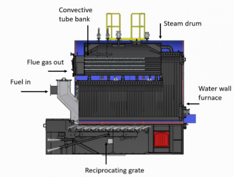
A hybrid boiler consists of a combustion chamber surrounded by a water tube heat transfer panel and a boiler drum with a set of convection heat transfer tubes as shown in Figure 1. Hot flue gas generated in the combustion chamber transfers heat to the water wall panel and enters the convection tubes placed inside the boiler drum.
The water tube heat transfer panel receives water from the drum through the downcomer. Riser tubes of furnace heat transfer panel receive heat from flue gas to generate water and steam mixture, which rises to the steam drum due to buoyancy effect. Drum water also receives heat from flue gas through the fire tube convection heat transfer surface. The boiler drum receives feed water and supplies steam to process.
Figure 1. Constructional details of the coal-fired hybrid boiler
2.1 Combustion modelling
Solid fuel combustion passes through various stages like drying, volatile generation, volatile combustion, and char combustion. Figure 1 shows the reciprocating grate as a combustor, where fuel is pushed in different zones by the reciprocating action of the grate. As it has a significant delay in combustion, it is difficult to correlate the rate of fuel firing and heat generation. Combustion delay is quite high in fuel like coal with a lower percentage of the volatile and higher percentage of char, as char combustion is a very slow process. A good combustion model involves heat transfer, evaporation, devolatilization, and char combustion. This makes the model quite complex. It also reduces the usability of the model due to its strong correlation with fuel ingredients and expected variation in fuel. A data-driven model can be used for the prediction of the combustion behaviour of the fuel.
If a fuel particle spends ‘t’ second over the grate before getting transferred to the ash removal system, cumulative heat generation can be approximated as follows.
$Q_{\text {cgen }}=m_{p} L H V\left(a-b e^{-c t}\right)$ (1)
where, mp is the mass of the fuel particle and LHV is the low heat value of the fuel. a, b and c are the coefficients.
Eq. (1) is modified by dividing the total time in multiple time steps and cumulative fractional heat generation by a mass of fuel after ith time step can be expressed as follows.
$Y_{i}=W_{1}-W_{2} e^{-W_{3} i}$ (2)
where W1, W2 and W3 are coefficients and can be calculated by using regression analysis. Cumulative fractional heat generation is the ratio of cumulative heat generation and the product of lower heat value and mass of the fuel.
Fractional heat generation for the first time step can be calculated as follows.
$\Delta Y_{1}=W_{1}-W_{2} e^{-W_{3}}$ (3)
Fractional heat generation for the other time steps can be calculated as the difference of cumulative fractional heat generation of ith time step and cumulative fractional heat generation of i-1th time step.
$\Delta Y_{i}=Y_{i}-Y_{i-1}$ (4)
If any fuel particle spends ‘M’ time steps over a reciprocating grate, a grate contains fuels of each time step and total heat generation can be expressed as a summation of heat generation of fuels of different time steps.
$Q_{g e n}=\sum_{i}^{M} m f_{i} \Delta Y_{i} L H V$ (5)
where mfi represent the mass of the fuel, which has spent ith time over the grate.
2.2 Heat transfer analysis
Total heat generated in the boiler is not transferred to the water for steam generation, a significant portion of the total heat is lost to the atmosphere as stack loss. Heat transfer to water and steam mixture through heat transfer surface is expressed as follows.
$Q_{T}=W_{4} Q_{g e n}$ (6)
where W4 represents the heat transfer efficiency.
Total heat transfer in the boiler is distributed between the furnace and the convective tube bank. Heat transfer distribution among furnace and convective tube banks is an important parameter for the analysis of boiler dynamics. Fractional heat transfer in the furnace can be expressed as a function of load with a polynomial equation.
$X_{F}=W_{5}+W_{6}$ Load $+W_{7}$ Load $^{2}$ (7)
where, W5, W6, and W7 are the coefficients and can be calculated by using regression analysis.
Heat transfer in the furnace is calculated as follows.
$Q_{F}=X_{F} Q_{T}$ (8)
Similarly, heat transfer in the convective bank can be calculated as follows.
$Q_{C}=X_{C} Q_{T}$ (9)
where, XC is the fractional heat generation in convective tube bank and can be calculated as follows.
$X_{C}=1-X_{F}$ (10)
2.3 Boiler dynamics
For simplification, the boiler can be divided into three parts: water circulation circuit consisting of downcomer and riser tubes of furnace water tube panel, drum below the water level and drum above the water level. Unlike a water tube boiler, complete heat transfer does not take place in riser tubes and heat transfer distribution between furnace and convection tube section is calculated for drum modelling.
2.3.1 Water circulation circuit
The water circulation circuit consists of downcomer and evaporator tubes. Downcomer receives the saturated water from steam drum and the saturated water enters the evaporator tubes, where it receives the heat from the flue gas and the evaporation of water takes place. Water and steam mixture in evaporator rises due to buoyancy force and enters to the steam drum. Mass, energy, and momentum conservation equations are required to understand and analyse the behaviour of the natural circulation circuit.
Mass conservation equation of natural circulation circuit is represented by the following equation.
$\frac{d}{d t}\left(\rho_{s} \overline{\alpha_{v}} V_{r}+\rho_{w}\left(1-\overline{\alpha_{v}}\right) V_{r}+\rho_{w} V_{d c}\right)=q_{d c}-q_{r}$ (11)
where, qdc is the saturated water flow from steam drum to downcomer and qr is the flow of water and steam mixture from riser to steam drum. Vr and Vdc are the volumes of risers and downcomers.
Mass conservation equation of natural circulation circuit can be further simplified as follows.
$\begin{aligned} {\left[V_{r} \overline{\alpha_{v}} \frac{d \rho_{s}}{d p}+\{(1-\right.} &\left.\left.\overline{\alpha_{v}}\right) V_{r}+V_{d c}\right\} \frac{d \rho_{w}}{d p} \left.+\left(\rho_{s} V_{r}-\rho_{w} V_{r}\right) \frac{d \overline{\alpha_{v}}}{d p}\right] \frac{d p}{d t}+\left(\rho_{s} V_{r}-\rho_{w} V_{r}\right) \frac{d \overline{\alpha_{v}}}{d \alpha_{r}} \frac{d \alpha_{r}}{d t}+q_{r} =q_{d c} \end{aligned}$ (12)
$\overline{\alpha_{v}}$ is the average void fraction in the riser and is calculated by the following [5].
$\overline{\alpha_{v}}=\frac{\rho_{w}}{\rho_{w}-\rho_{s}}\left[1-\frac{\rho_{s}}{\alpha_{r}\left(\rho_{w}-\rho_{s}\right)} \ln \left(1+\frac{\rho_{w}-\rho_{s}}{\rho_{s}} \alpha_{r}\right)\right]$ (13)
where αr is the dryness fraction at the outlet of riser tubes.
The following equation represents the energy conservation equation for the natural circulation circuit.
$\frac{d}{d t}\left\{\rho_{s} \cdot h_{s} \overline{\alpha_{v}} \cdot V_{r}+\rho_{w} h_{w}\left(\left(1-\overline{\alpha_{v}}\right) V_{r}+V_{d c}\right)-p V_{r}\right\}=Q_{F}+q_{d c} h_{w}-\left(\alpha_{r} h_{c}+h_{w}\right) q_{r}$ (14)
where hc is the difference between saturated vapour and saturated liquid enthalpy and is referred to as condensation enthalpy.
The energy conservation equation of the natural circulation circuit can be simplified as follows.
$\begin{aligned}\left\{\overline{\alpha_{v}} V_{r}\left(h_{s} \frac{d \rho_{s}}{d p}+\right.\right.&\left.\rho_{s} \frac{d h_{s}}{d p}\right) +\left(\left(1-\overline{\alpha_{v}}\right) V_{r}+V_{d c}\right)\left(h_{w} \frac{d \rho_{w}}{d p}\right.\left.+\rho_{w} \frac{d h_{w}}{d p}\right) +\left(\rho_{s} h_{s} V_{r}-\rho_{w} h_{w} V_{r}\right) \frac{d \overline{\alpha_{v}}}{d p} \left.-V_{r}\right\} \frac{d p}{d t} +\left(\rho_{s} h_{s} V_{r}-\rho_{w} h_{w} V_{r}\right) \frac{d \overline{\alpha_{v}}}{d \alpha_{r}} \frac{d \alpha_{r}}{d t} +\left(\alpha_{r} h_{c}+h_{w}\right) q_{r}=Q_{F}+q_{d c} h_{w} \end{aligned}$ (15)
In a natural circulation loop, water flow in the downcomer takes place due to density differences in the downcomer and riser column. This is calculated by using the momentum balance equation of the natural circulation loop. Elgandelwar et al. [15] present a steady-state model using a momentum balance equation for the flow distribution analysis in natural circulation. The following equation represents the momentum balance equation of a natural circulation loop in a water tube or hybrid boiler [6].
$\left(\rho_{w}-\rho_{s}\right) \overline{\alpha_{v}} V_{r} g-\frac{k_{d c} q_{d c}{ }^{2}}{2 \rho_{w} A_{d c}}=0$ (16)
where kdc is a dimensionless number, which depends on the friction factor and geometry of the boiler and Adc is the area of the downcomer.
Normally a constant value of kdc is used for the dynamic simulation of a boiler but the dryness fraction of the riser has a great influence on this dimensionless number. It can be expressed as a function of dryness fraction at the outlet of the riser tube as follows.
$k_{d c}=W_{8}+W_{9} \alpha_{r}+W_{10} \alpha_{r}^{2}$ (17)
where W8, W9 and W10 are coefficients and calculated by regression analysis.
2.3.2 Drum below water level
For simplification, the drum is divided into two volumes: drum below the water level and drum above the water level. Drum volume below the water level receives feed water and supplies steam to the upper section of the drum. It also receives water and steam mixture from riser tubes and supplies saturated water to the downcomer pipes. If the steam generation in the drum is higher than the steam required in the process, pressure and the corresponding saturation temperature of the drum increases receiving heat from the steam and causing the condensation of steam. If the steam generation in the drum is less than the process requirement, pressure and corresponding saturation temperature decreases rejecting heat to the drum water and causing evaporation of the steam. To model this phenomenon, qcd term is introduced to represent the rate of condensation in the steam drum. A negative rate of condensation indicates the flashing of steam. To understand and analyse the phenomenon in the drum below the water level, two separate mass conservation equations for water and steam are required in addition to a combined energy equation.
The following equation represents the steam mass conservation equation in the steam drum below the water level.
$\frac{d}{d t}\left(\rho_{s} V_{d w} \varphi\right)=\alpha_{r} q_{r}-q_{s d}-q_{c d}$ (18)
where, Vdw is total drum volume below the water level and ф is the volume fraction occupied by steam. qcd is the rate of steam condensation and qsd is the steam flow to the upper section of the drum. Steam mass conservation equation of steam drum below water level can be further simplified as follows.
$V_{d w} \varphi \frac{d \rho_{s}}{d t}+\rho_{s} \varphi \frac{d V_{d w}}{d t}+\rho_{s} V_{d w} \frac{d \varphi}{d t}=\alpha_{r} q_{r}-q_{s d}-q_{c d}$ (19)
$V_{d w} \varphi \frac{d \rho_{s}}{d p} \frac{d p}{d t}+\rho_{s} \varphi \frac{d V_{d w}}{d t}+\rho_{s} V_{d w} \frac{d \varphi}{d t}-\alpha_{r} q_{r}+q_{s d}+q_{c d}=0$ (20)
Similar to the steam mass conservation equation, water mass conservation can be also written for the drum below the water level.
$\frac{d}{d t}\left\{\rho_{w} V_{d w}(1-\varphi)\right\}=\left(1-\alpha_{r}\right) q_{r}+q_{c d}+q_{f}-q_{d c}$ (21)
qf is the mass of feedwater flow rate to the boiler drum. The water mass conservation equation can be simplified as follows.
$\begin{aligned} V_{d w}(1-\varphi) \frac{d \rho_{w}}{d p} & \frac{d p}{d t}+\rho_{w}(1-\varphi) \frac{d V_{d w}}{d t}-\rho_{w} V_{d w} \frac{d \varphi}{d t}-\left(1-\alpha_{r}\right) q_{r}-q_{c d} =q_{f}-q_{d c} \end{aligned}$ (22)
Energy equation can be combined for water and steam in the drum below the water level, as it involves phase change and heat transfer across the phase. The following equation represents the energy equation for drum volume below water level.
$\begin{aligned} \frac{d}{d t}\left\{\rho_{s} V_{d w} \varphi h_{s}+\right.& \rho_{w} V_{d w}(1-\varphi) h_{w}+m_{d r u m} C_{m} T_{s} \left.-P V_{d w}\right\} =Q_{C}+\left(\alpha_{r} q_{r}-q_{s d}\right) h_{s} +\left\{\left(1-\alpha_{r}\right) q_{r}-q_{d c}\right\} h_{w}+q_{f} h_{f} \end{aligned}$ (23)
Similar to other equations, this equation can be expanded and the final equation can be written as follows.
$\begin{aligned}\left\{V_{d w} \varphi\left(h_{s} \frac{d \rho_{s}}{d p}+\right.\right.&\left.\rho_{s} \frac{d h_{s}}{d p}\right) +V_{d w}(1-\varphi)\left(h_{w} \frac{d \rho_{w}}{d p}\right.\left.+\rho_{w} \frac{d h_{w}}{d p}\right)+m_{d r u m} C_{m} \frac{d T_{s}}{d p}\left.-V_{d w}\right\} \frac{d p}{d t}+\left\{\rho_{s} h_{s} \varphi+\rho_{w} h_{w}(1-\varphi)\right.\\ &-p\} \frac{d V_{d w}}{d t}+\left\{\rho_{s} h_{s} V_{d w}-\rho_{w} V_{d w} h_{w}\right\} \frac{d \varphi}{d t}-\left\{\alpha_{r} h_{s}+\left(1-\alpha_{r}\right) h_{w}\right\} q_{r} +h_{s} q_{s d}=Q_{C}-q_{d c} h_{w}+q_{f} h_{f} \end{aligned}$ (24)
2.3.3 Steam mass flow
Steam flows from the lower section of the drum to the upper section of the drum because of the buoyancy effect. Many different models have been attempted for the calculation of steam mass flow rate qsd. Astrom et al. [6] has presented an empirical model for the calculation. Oritz [10] has also attempted an empirical model for the simulation of a fire tube boiler. Kim et al. [8] and Adam et al. [7] use the drift velocity formula for the calculation of steam separation velocity. The following equation [16] is used for the calculation of drift velocity in the boiler drum.
$u_{s}=1.41\left\{\frac{\eta g\left(\rho_{w}-\rho_{s}\right)}{\rho_{w}{ }^{2}}\right\}^{1 / 4}$ (25)
Asep represents the steam separation area. As the complete steam separation area is not used for the steam separation. It can be multiplied by ф to consider the area of steam separation surface occupied by the steam, as ф represents the fraction of volume in the drum below water level occupied by steam.
$q_{s d}=A_{\operatorname{sep}} \varphi u_{s} \rho_{s}$ (26)
2.3.4 Steam drum above water level
As it contains single-phase steam, it requires only one mass conservation equation for steam to represent the phenomenon. The following equation represents the mass conservation equation in the drum volume above water level.
$\frac{d}{d t}\left(\rho_{s} V_{d s}\right)=q_{s d}-q_{s}$ (27)
where Vds is the volume of the drum above water level and qs is the steam flow to the process. This can be expanded as follows.
$V_{d s} \frac{d \rho_{s}}{d t}+\rho_{s} \frac{d V_{d s}}{d t}=q_{s d}-q_{s}$ (28)
As the total volume of the drum is constant, it can be written as follows.
$V_{d w}+V_{d s}=c$ (29)
After differentiation, it yields to the following equation.
$\frac{d V_{d w}}{d t}=-\frac{d V_{d s}}{d t}$ (30)
Eq. (30) is used for the substitution of $\frac{d V_{d s}}{d t}$ by $\frac{d V_{d w}}{d t}$ in Eq. (28). This results in the following equation.
$V_{d s} \frac{d \rho_{s}}{d p} \frac{d p}{d t}-\rho_{s} \frac{d V_{d w}}{d t}-q_{s d}=-q_{s}$ (31)
2.3.5 Integrated Model for drum dynamics of boiler
Eqns. (12), (15), (20), (22), (24), (26) & (31) represent the final equations in terms of desired variables $\frac{d p}{d t}, \frac{d V_{w}}{d t}, \frac{d \varphi}{d t}, \frac{d \alpha_{r}}{d t}, q_{r}, q_{s d}, q_{c d}$ for model development. These equations are simultaneously solved to predict the boiler drum dynamics. These equations and variables are numbered from 1 to 7. Coefficients of the different variables are specified as Cij, where i represents equation number and j represents a variable number. The left side constant of the equation is specified as di, where i represents the equation number.
Eq. (12) represent the mass conservation equation for the natural circulation circuit and can be specified as equation number 1. Eq. (12) can be written as follows.
$\begin{aligned} {\left[V_{r} \overline{\alpha_{v}} \frac{d \rho_{s}}{d p}+\{(1\right.} &\left.\left.-\overline{\alpha_{v}}\right) V_{r}+V_{d c}\right\} \frac{d \rho_{w}}{d p}\left.+\left(\rho_{s} V_{r}-\rho_{w} V_{r}\right) \frac{d \overline{\alpha_{v}}}{d p}\right] \frac{d p}{d t}+\left(\rho_{s} V_{r}-\rho_{w} V_{r}\right) \frac{d \overline{\alpha_{v}}}{d \alpha_{r}} \frac{d \alpha_{r}}{d t}+q_{r} =q_{d c} \end{aligned}$
This equation can be rewritten as follows.
$C_{11} \frac{d p}{d t}+C_{12} \frac{d V_{d w}}{d t}+C_{13} \frac{d \varphi}{d t}+C_{14} \frac{d \alpha_{r}}{d t}+C_{15} q_{r}+C_{16} q_{s d}+C_{17} q_{c d}=d_{i}$ (32)
where all the coefficients can be calculated as follows.
$C_{11}=V_{r} \overline{\alpha_{v}} \frac{d \rho_{s}}{d p}+\left(V_{r}\left(1-\overline{\alpha_{v}}\right)+V_{d c}\right) \frac{d \rho_{w}}{d p}+\left(\rho_{s} V_{r}-\rho_{w} V_{r}\right) \frac{d \overline{\alpha_{v}}}{d p}$
$C_{12}=0$
$C_{13}=0$
$C_{14}=\left(\rho_{s} V_{r}-\rho_{w} V_{r}\right) \frac{d \overline{\alpha_{v}}}{d \alpha_{r}}$
$C_{15}=1$
$C_{16}=0$
$C_{17}=0$
$d_{1}=q_{d c}$
Downcomer flow (qdc) is calculated by using Eq. (16). Other equations can be also rewritten in the same form and a generalized equation can be deduced as follows.
$C_{i 1} \frac{d p}{d t}+C_{i 2} \frac{d V_{d w}}{d t}+C_{i 3} \frac{d \varphi}{d t}+C_{i 4} \frac{d \alpha_{r}}{d t}+C_{i 5} q_{r}+C_{i 6} q_{s d}+C_{i 7} q_{c d}=d_{i}$ (33)
where, i represent the equation number. A system of the equation can be developed and arranged in a matrix as follows.
$\left[\begin{array}{lllllll}C_{11} & C_{12} & C_{13} & C_{14} & C_{15} & C_{16} & C_{17} \\ C_{21} & C_{22} & C_{23} & C_{24} & C_{25} & C_{26} & C_{27} \\ C_{31} & C_{32} & C_{33} & C_{34} & C_{35} & C_{36} & C_{37} \\ C_{41} & C_{42} & C_{43} & C_{44} & C_{45} & C_{46} & C_{47} \\ C_{51} & C_{52} & C_{53} & C_{54} & C_{55} & C_{56} & C_{57} \\ C_{61} & C_{62} & C_{63} & C_{64} & C_{65} & C_{66} & C_{67} \\ C_{71} & C_{72} & C_{73} & C_{74} & C_{75} & C_{76} & C_{77}\end{array}\right]\left[\begin{array}{c}d p / d t \\ d V_{d w} / d t \\ d \varphi / d t \\ d \alpha_{r} / d t \\ q_{r} \\ q_{s d} \\ q_{c d}\end{array}\right] =\left[\begin{array}{l}d_{1} \\ d_{2} \\ d_{3} \\ d_{4} \\ d_{5} \\ d_{6} \\ d_{7}\end{array}\right]$
2.3.6 Integrated model
An integrated model for drum dynamics requires input like water side heat transfer in the furnace, waterside heat transfer in convection tube bank and downcomer flow. A set of empirical equations are used for the calculation of heat generation (Eqns. (2) to (5)), waterside heat transfer in the furnace (Eqns. (6) to (10)), waterside heat transfer in convection bank (Eqns. (6) to (10)), the dimensionless parameter for the calculation of downcomer flow (Eq. (17)). These equations are represented as a function of 10 coefficients (W1 to W10) as variables. These equations are used for the calculation of required parameters like water side heat transfer in the furnace, waterside heat transfer in convection bank and downcomer flow for the integrated boiler dynamics model. Integrated boiler dynamics is used for the prediction of pressure and water level at different time steps. Predicted and actual values of pressure and water level are compared to estimate errors. The objective of this model is to minimise errors by identifying the optimum set of variables.
The following equations are used for the calculation of the errors in pressure and water level estimation.
$\operatorname{ErP}_{i}=p a_{i}-p m_{i}$ (34)
$E r L_{i}=L a_{i}-L m_{i}$ (35)
where ErPi and ErLi are errors in pressure and water level. Pai and Pmi are actual and predicted values of pressure respectively. Lai and Lmi are actual and predicted values of water level respectively.
This is the case of multi-objective optimisation as both errors in pressure and water level need to be minimised. Weighted sum method and least square technique are used, where both objectives are combined in a single objective function by adding them after multiplying the square of errors and weightage as follows.
$\operatorname{Er}=X_{p} \sum_{i}^{N} \operatorname{Er} P_{i}^{2}+X_{L} \sum_{i}^{N} \operatorname{Er} L_{i}{ }^{2}$ (36)
where, XP and XL are weightage of pressure and level errors.
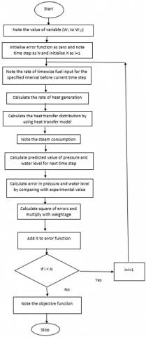
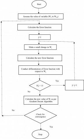
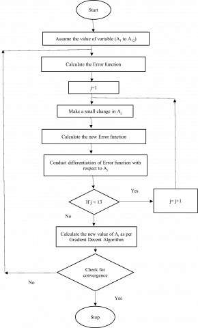
The batch gradient descent method can be used for the minimisation of the error function (Er). Initial values of the various coefficient variables (W1 to W10) are assumed. The rate of combustion, heat transfer, distribution of heat transfer and downcomer flow are calculated. The boiler dynamics model is used to predict pressure and water level. Model output is compared with the experimental data to compare errors in pressure and water level for each time step. The final error function is calculated by using Eq. (36). A small change in each variable is introduced to calculate the new value of the error function and gradients are calculated. The new set of coefficient variables is calculated by using the gradient descent algorithm. The stepwise calculation has been explained by flowcharts in Figure 2a and Figure 2b.
(a)
(b)
Figure 2. (a) Flow chart for the calculation of error function; (b) Flow chart for the minimisation of the error function
2.4 Extension of the integrated model for the prediction of flue gas composition
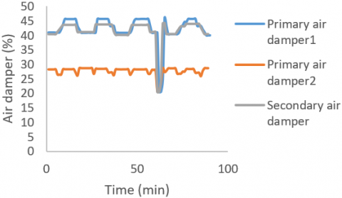
The air to fuel ratio in grate combustion is controlled by multiple air dampers. Damper position and fuel firing rate in a grate boiler are controlled by a control table, where damper positions and fuel firing are tabulated as a function of boiler load. It is quite difficult to operate coal-fired grate boiler at optimum air to fuel ratio due to significant combustion lag in coal combustion. If the integrated model is used for the prediction of the rate of combustion, it is possible to analyse the characteristics of air damper and predict the air quantity and oxygen level in the flue gas. In the test boiler, two primary air dampers and one secondary air damper are used.
The following equations can be used for the estimation of air quantity for each damper.
$m a_{1}=A_{1}+A_{2} D_{1}+A_{3} D_{1}^{2}+A_{4} D_{1}^{3}$ (37)
$m a_{2}=A_{5}+A_{6} D_{2}+A_{7} D_{2}^{2}+A_{8} D_{2}^{3}$ (38)
$m a_{3}=A_{9}+A_{10} D_{3}+A_{11} D_{3}^{2}+A_{12} D_{3}^{3}$ (39)
where, D1, D2 and D3 are the damper position and A1 to A12 are the coefficients of the polynomial equations.
Total air quantity is calculated as the sum of the air quantity for each damper.
$m a=m a_{1}+m a_{2}+m a_{3}$ (40)
Eq. (5) is used for the rate of heat generation and the rate of combustion can be calculated by dividing heat generation by LHV. Flue gas composition is calculated by using total air quantity and rate of combustion. Oxygen percentage in dry flue gas is calculated and compared with the measured value of oxygen. The following equation is used for the calculation of error in oxygen.
$\operatorname{Ero}_{i}=o a_{i}-o m_{i}$ (41)
Mean squared error in prediction in oxygen level is expressed as follows.
$M S E r o=\frac{1}{N} \sum_{i}^{N} \operatorname{Ero}_{i}^{2}$ (42)
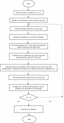
Mean squared errors in oxygen prediction is minimised by using the Batch Gradient Descent algorithm for the calculation of the optimum set of coefficient variables. Figure 3a and Figure 3b present flowcharts for the calculation and minimisation of the error function.
(a)
(b)
Figure 3. (a) Flow chart for the calculation of error function; (b) Flow chart for the minimisation of the error function
Analysis has been conducted for an 8 TPH coal-fired hybrid boiler with the following design details in Table 1.
Table 1. Design and construction details of boiler
|
S. No. |
Description |
Value |
Unit |
|
1 |
Boiler capacity |
8000 |
kg/h |
|
2 |
Fuel |
Coal |
|
|
3 |
Combustor |
Reciprocating grate |
|
|
4 |
LHV |
24244 |
kJ/kg |
|
5 |
Riser volume |
0.872685 |
m3 |
|
6 |
Downcomer area |
0.035343 |
m2 |
|
7 |
Drum volume |
7.381298 |
m3 |
|
8 |
Steam separation area |
6.016384 |
m2 |
3.1 Model input
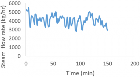
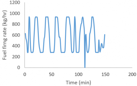
Steam flow rate and fuel firing rate has been recorded for 150 minutes. Steam flow rate and fuel firing rate have been plotted as a function of time in Figure 4 and Figure 5 respectively. Steam flow rate and fuel firing rate provide input for the model development.
Figure 4. Steam flow rate as a function of time
Figure 5. Fuel firing rate as a function of time
3.2 Model development
Total time spent by fuel on the reciprocating grate changes as a function of grate speed. Fuel layer velocity on grate has been recorded as 9 m/hr and the grate length is 4.6 m. The average time spent by a fuel particle on the grate can be approximated as 30 minutes. At any moment of time grate contains fuel entering to furnace within 30 minutes and these fuels are at different stages of combustion. Model is trained for the data between 31 minutes to 90 minutes as initial 30 minutes data of fuel firing are required for the prediction of the rate of combustion and heat transfer distribution.
All variables are initialised and rate of combustion, heat transfer in furnace, heat transfer in convection bank and downcomer flow are calculated at each time step and boiler dynamics model is used to predict pressure and water level. Pressure and water level of experimental data and predicted value are compared to calculate error in pressure (ErPi) and error in water level (ErLi). As level has been presented in percentage and pressure is presented in bar, ErLi dominates over ErPi and skew error function. It requires normalisation of error in water level. Eq. (36) can be normalised as follows.
$\operatorname{Er}=X_{p} \sum_{i}^{N} \operatorname{Er} P_{i}^{2}+\frac{X_{L}}{100} \sum_{i}^{N} \operatorname{Er} L_{i}^{2}$ (43)
Weightage for pressure error (XP) and weightage for water level (XL) are considered as 0.5.
Table 2. Optimum values of model variables
|
S. No. |
Variables |
Value |
|
1 |
W1 |
1.002 |
|
2 |
W2 |
0.981 |
|
3 |
W3 |
0.07252 |
|
4 |
W4 |
0.833 |
|
5 |
W5 |
0.416 |
|
6 |
W6 |
0.105 |
|
7 |
W7 |
0.053 |
|
8 |
W8 |
78.732 |
|
9 |
W9 |
4233.145 |
|
10 |
W10 |
554.013 |
The error function is minimised by using the batch gradient descent algorithm and a set of variables are deduced. Table 2 compiles all model variables and their deduced value on the converged solution.
Mean absolute error and relative mean absolute error are good indicators for the accuracy of the model. Mean absolute error (MAE) is calculated as follows.
$M A E=\frac{\sum_{1}^{N}\left(\left|y a_{i}-y m_{i}\right|\right)}{N}$ (44)
where yai and ymi are the experimental result and model output of a parameter respectively. N is the number of the data point.
The relative mean absolute error can be used to test the accuracy of the model. The relative mean absolute error can be calculated as follows.
$R M A E=\left(\frac{M A E}{\overline{y a}}\right) 100 \%$ (45)
where $\overline{y a}$ is the mean of experimental values.
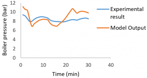
Figure 6 shows the comparison of experimental results and predicted output of boiler pressure. Timewise variation in the predicted value of pressure almost follows the experimental result. RMAE for pressure estimation has been calculated as 8.4%.
Figure 6. Pressure as a function of time for training data
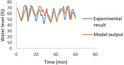
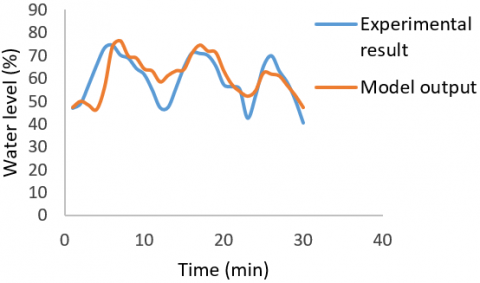
Figure 7 shows the comparison of experimental results and predicted output of boiler water level. It shows the predicted value of water level variation almost follows the experimental result. RMAE for water level prediction has been calculated as 8.88%.
Figure 7. Water level as a function of time for training data
3.3 Model validation
One hour of data has been used for the model training and it has been tested for the next half hour to check the predictability of the model. Figure 8 shows the comparison of experimental result and model output for the pressure. RMAE has been calculated for the pressure and has been estimated as 13.05%. It is comparatively higher than the previous set of data, as regression has been also conducted with the previous set of data. Figure 9 shows the comparison of experimental results and model output for the water level. A similar analysis has been conducted for water level and RMAE has been calculated as 8.72%. Predictability of water level has been found a little better compared to the predictability of pressure.
Figure 8. Pressure as a function of time for test data
Figure 9. Water level as a function of time for test data
3.4 Prediction of oxygen
As the air to fuel ratio is controlled by the position of air dampers, air damper positions provide input variables. Figure 10 provides the air damper position as a function of time.
Eqns. (37)-(40) are used to calculate air quantity and Eq. (5) is used for the calculation of the rate of combustion. The stoichiometric calculation is conducted to calculate the predicted value of oxygen level and is compared with the experimental value. The difference of the predicted level of oxygen and experimental value is calculated as the error and mean squared errors is calculated by using Eq. (42). The mean squared error is minimised for the training data set by using the Batch Gradient Descent algorithm.
Figure 10. Damper position as a function of time
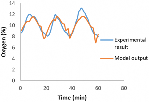
Table 3 compiles all model variables and their deduced value on the converged solution. Initial one hour data is chosen for training and the next half hour data is used for testing of the model. Figure 11 shows the comparison of timewise variation of predicted oxygen level and the experimental oxygen level. It shows that the predicted value of oxygen almost follows the experimental result. RMAE for the training data has been calculated as 6.15%.
Table 3. Optimum values of model variables for oxygen prediction
|
S. No. |
Variables |
Value |
|
1 |
A1 |
0.1000 |
|
2 |
A2 |
0.1000 |
|
3 |
A3 |
0.1001 |
|
4 |
A4 |
0.0733 |
|
5 |
A5 |
0.1000 |
|
6 |
A6 |
0.1000 |
|
7 |
A7 |
0.0979 |
|
8 |
A8 |
0.0051 |
|
9 |
A9 |
0.1000 |
|
10 |
A10 |
0.1000 |
|
11 |
A11 |
0.0994 |
|
12 |
A12 |
0.0376 |
Figure 11. Oxygen level as a function of time for training data
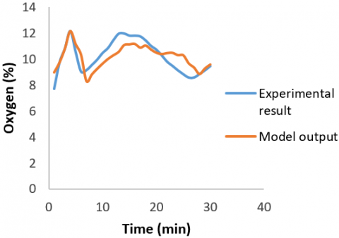
Figure 12. Oxygen level as a function of time for test data
Figure 12 shows the comparison of timewise variation of predicted oxygen level and the experimental oxygen level for the test data. RMAE has been calculated for test data as 6.15%.
The boiler dynamics of a hybrid boiler is quite different from a water tube boiler as heat transfer is distributed in the water tube furnace and fire tube convection surface. As heat transfer takes place in the boiler drum, it makes the hydrodynamic analysis more complex in comparison with the water tube boiler. It is easy to estimate heat generation and heat transfer in an oil and gas fired boiler, as combustion is instantaneous and directly calculated from the fuel firing rate. In a solid fuel fired boiler, a fuel particle passes through the different stages of combustion and releases heat differently at different times depending on the stage of combustion. It requires a complex model for the prediction of heat generation. The predictability of this model is quite less due to variability in fuel properties and composition. A simplified data-driven model is used for the prediction of heat generation, heat transfer and distribution of heat transfer among furnace and convective tubes. This model can capture the variability of fuel and its effect on heat release patterns. This model can also predict the variation in heat transfer due to slagging and fouling of the heat transfer surface. This model is integrated with the hydrodynamic model. The hydrodynamic model divides the boiler into three zones: riser downcomer circuit for a furnace water wall, drum below water level and drum above water level. Mass and energy conservation equations are developed for these three zones and a separate equation for steam separation has been added to the model.
An integrated combustion, heat transfer and hydrodynamic model is used to predict the pressure and water level in the boiler. The predicted value is compared with the experimental value to identify errors and the multi-objective function optimisation strategy is used for the minimisation of errors. Model is developed for 60 minutes to identify the optimum set of variables and used to test the accuracy of the model for the next 30 minutes of data. The root mean absolute error method presents a simplified approach for the estimation of the accuracy of the model. It shows the RMAE value as 13.05% and 8.72% in the estimation pressure and water level respectively. This model can be extended for the control of pressure and water level of a coal-fired reciprocating grate boiler in extremely fluctuating load conditions.
The model has been extended for the prediction of oxygen level, where the mass flow rate of combustion air is calculated and the predicted value of the rate of combustion is used for the estimation of oxygen level in the flue gas. It shows an RMAE of 6.15% for the test data. Oxygen level indicates the air to fuel ratio and plays a significant role in efficient fuel combustion and emission control. This model can be extended for the control of pressure, water level and air to fuel ratio for the efficient and safe operation of a coal-fired boiler.
The authors are extremely thankful to Mr. Rakesh Tripathi & Mr. K. P. Harigovind for their continuous support and encouragement. Also, the support from Mr. Abhay Mane and Mr. N. V. Kate during the research work are gratefully acknowledged.
|
a |
Coefficient |
|
Adc |
Downcomer area, m2 |
|
Ai |
Model variable for oxygen prediction |
|
Asep |
Separation area, m2 |
|
b |
Coefficient |
|
c |
Coefficient |
|
Cij |
Coefficient for generalized matrix for ith equation jth variable |
|
Cm |
Specific heat of riser & drum material, J/kgK |
|
Di |
Air damper position of ith damper (%) |
|
di |
Right side constant for ith equation |
|
Er |
Square of errors |
|
Eroi |
Error in oxygen at ith time step |
|
ErLi |
Error in level at ith time step |
|
ErPi |
Error in pressure at ith time step |
|
g |
Gravitational acceleration, m/s2 |
|
hc |
Condensation enthalpy, J/kg |
|
hf |
Feed water enthalpy, J/kg |
|
hs |
Saturated Vapour enthalpy, J/kg |
|
hw |
Saturated Liquid enthalpy, J/kg |
|
kdc |
Dynamic coefficient for natural circulation |
|
Lai |
circuit |
|
LHV |
Actual % level at ith time step |
|
Lmi |
Low heat value, J/kg |
|
N |
Model % level at ith time step |
|
MAE |
Number of time steps in combustion model |
|
ma |
Minimum absolute error |
|
mai |
Combustion air mass flow rate |
|
mdrum |
Air mass flow rate through ith damper |
|
mfi |
Mass of drum, kg |
|
mp |
Fuel input at ith time step, kg |
|
MSEro |
Mass of fuel particle, kg |
|
N |
Mean squared error in oxygen prediction |
|
oai |
Number of time steps in training data |
|
omi |
Actual oxygen at ith time step |
|
p |
Model oxygen at ith time step |
|
Pai |
Pressure, Pa |
|
Pmi |
Actual pressure at ith time step |
|
QC |
Model pressure at ith time step |
|
Qcgen |
Heat transfer in convection bank, W |
|
QF |
Cumulative heat generation, W |
|
Qgen |
Heat transfer in the furnace, W |
|
QT |
Cumulative heat generation, W |
|
qcd |
Total Heat transfer, W |
|
qdc |
Rate of condensation, kg/s |
|
qf |
Downcomer flow rate, kg/s |
|
qr |
Feedwater flow rate, kg/s |
|
qs |
Riser flow rate, kg/s |
|
qsd |
Steam flow rate to process, kg/s |
|
RMAE |
Relative mean absolute error |
|
t |
time, s |
|
Ts |
Saturation temperature, K |
|
us |
Drift velocity, m/s |
|
Vdc |
Downcomer volume, m3 |
|
Vdw |
Drum volume below water level, m3 |
|
Vds |
Drum volume above water level, m3 |
|
Vr |
Riser volume, m3 |
|
Wi |
Model variables |
|
XC |
Fractional heat transfer in convective bank |
|
XF |
Fractional heat transfer in the furnace |
|
XL |
Weightage of level error |
|
XP |
Weightage of pressure error |
|
Yi |
Cumulative fractional heat generation till ith time step |
|
yai |
Actual value of the parameter at ith time step |
|
ymi |
Model value of the parameter at ith time step |
|
$\overline{y a}$ |
Average value of the actual parameter |
|
Greek symbols |
|
|
ρ |
Density of tube and fin, kg/m3 |
|
ρs |
Saturated vapour density, kg/m3 |
|
ρw |
Saturated liquid density, kg/m3 |
|
αr |
Dryness fraction at the riser outlet |
|
$\overline{\alpha_{v}}$ |
Average void fraction in the riser tube |
|
Ф |
Steam volume fraction in the drum below water level |
|
ΔYi |
Fractional heat generation in ith time step |
|
$\eta$ |
Surface tension, N/m |
|
Subscripts |
|
|
dc |
Downcomer |
|
drum |
Drum |
|
ds |
Above water level |
|
dw |
Below water level |
|
i |
Time step |
|
r |
Riser |
|
s |
Vapour |
|
w |
Liquid |
[1] Tyss, A. (1981). Modelling and parameter estimation of a ship boiler. Automatica, 17(1): 157-166. https://doi.org/10.1016/0005-1098(81)90091-1
[2] Åström, K.J., Eklund, K. (1972). A simplified non-linear model of a drum boiler-turbine unit. International Journal of Control, 16(1): 145-169. http://dx.doi.org/10.1080/00207177208932249
[3] Åström, K.J., Bell, R.D. (1989). Simple drum-boiler models. In Power Systems: Modelling and Control Applications, pp. 123-127. https://doi.org/10.1016/B978-0-08-036135-2.50028-4
[4] Åström, K.J., Bell, R.D. (1993). A nonlinear model for steam generation processes. IFAC Proceedings Volumes, 26(2): 649-652. https://doi.org/10.1016/S1474-6670(17)48549-1
[5] Bell, R.D., Åström, K.J. (1996). A fourth order non-linear model for drum-boiler dynamics. IFAC Proceedings Volumes, 29(1): 6873-6878. https://doi.org/10.1016/S1474-6670(17)58787-X
[6] Åström, K.J., Bell, R.D. (2000). Drum-boiler dynamics. Automatica, 36(3): 363-378. http://dx.doi.org/10.1016/S0005-1098(99)00171-5
[7] Adam, E.J., Marchetti, J.L. (1999). Dynamic simulation of large boilers with natural recirculation. Computers & Chemical Engineering, 23(8): 1031-1040. https://doi.org/10.1016/S0098-1354(99)00269-0
[8] Kim, H., Choi, S. (2005). A model on water level dynamics in natural circulation drum-type boilers. International Communications in Heat and Mass Transfer, 32(6): 786-796. https://doi.org/10.1016/j.icheatmasstransfer.2004.10.010
[9] Tawfeic, S.R. (2013). Boiler drum-level modeling. Journal of Engineering Sciences, 41(5): 1812-1829. https://doi.org/10.21608/JESAUN.2013.114911
[10] Ortiz, F.G. (2011). Modeling of fire-tube boilers. Applied Thermal Engineering, 31(16): 3463-3478. https://doi.org/10.1016/j.applthermaleng.2011.07.001
[11] Miltner, M., Makaruk, A., Harasek, M., Friedl, A. (2006). CFD-modelling for the combustion of solid baled biomass. Parameters, 1(2): 1-6.
[12] Bauer, R., Gölles, M., Brunner, T., Dourdoumas, N., Obernberger, I. (2010). Modelling of grate combustion in a medium scale biomass furnace for control purposes. Biomass and Bioenergy, 34(4): 417-427. https://doi.org/10.1016/j.biombioe.2009.12.005
[13] Gölles, M., Bauer, R., Brunner, T., Dourdoumas, N., Obernberger, I. (2011). Model based control of a biomass grate furnace. In European Conference on Industrial Furnaces and Boilers, 9: 1-10.
[14] Boriouchkine, A., Jämsä-Jounela, S.L. (2016). Simplification of a mechanistic model of biomass combustion for on-line computations. Energies, 9(9): 735. https://doi.org/10.3390/en9090735
[15] Elgandelwar, A., Jha, R.S., Lele, M.M. (2020). Steady-state flow distribution analysis of natural circulation in water tube boiler. Computational Thermal Sciences: An International Journal, 12(3): 275-288. https://doi.org/10.1615/ComputThermalScien.2020033963
[16] Zuber, N., Findlay, J.A. (1965). Average volumetric concentration in two-phase flow systems. J. Heat Transfer., 87(4): 453-468. http://dx.doi.org/10.1115/1.3689137