I. Gede Tunas* | Yassir Arafat | Rudi Herman
© 2022 IIETA. This article is published by IIETA and is licensed under the CC BY 4.0 license (http://creativecommons.org/licenses/by/4.0/).
OPEN ACCESS
The present work aims to develop a flood peak equation because of data limitations due to the impact of damage to the streamflow measuring instrument as a result of the 2015 floods at an agricultural catchment in Sulawesi, Indonesia. Hydrologic data for the period 2002-2014 obtained from two hydrologic stations and one hydrometric station were applied to establish the research variables. Three variables were determined using the frequency analysis approach: design rainfall generated from partial duration series (RDP) and annual maximum series (RDA) of daily rainfall data, and design streamflow predicted from annual maximum series of daily streamflow data (QDA). Four types of frequency distributions are tested to determine those variables, consisting of Normal, Log Normal, Log Pearson Type III and Gumbel distributions. The third distribution was selected for determining all the variables with the largest difference in $\chi_{2}$ and $\Delta$ values based on Chi-squared and Kolmogorov–Smirnov tests respectively. The design streamflow equation that represents the peak of the flood was formulated by substituting the QDA with an equation generated from the regression analysis of those three variables. A streamflow peak equation was successfully developed as a function of RDP in the form of a power equation with excellent performance measured using Mean Absolute Error (MAE) and Correlation Coefficient (r). This equation could be applied in all of the catchments by accommodating the area's weighting factor of the sub-catchments.
extreme event, frequency analysis, flood forecasting, regression
One of the most important parts in hydrologic analysis related to water resource management in a catchment is data, particularly rainfall and streamflow data [1-3]. In general, both types of data can be obtained from various types of rainfall and streamflow measurement instruments installed in almost all areas of the globe for multipurpose. This instrument is basically installed in certain locations that are considered important for its management such as in agricultural, forest and settlement areas [4, 5]. However, the availability of the gauges is not spread evenly in various regions with several considerations such as the relatively expensive management costs and the difficulty of accessing the location if the gauges must be located in remote areas such as forests that are located very far from settlements [5, 6].
Technological developments have also been able to solve this problem, for example the use of rainfall radar or automatic rainfall and streamflow gauges to gather real time data [7]. The advantages of this instrument are not only the rapidity of data access but also the ability to record series data with very short time intervals such as minutes, hours and daily [8]. This type of data (rainfall) is spatially distributed so that it can present data with a wide area coverage. However, this type of instrument is installed in very limited quantities due to the very high investment, operation and maintenance costs.
Another concern is that the range of data is very limited and hence does not meet statistical requirements for parametric data analysis [9]. This limitation can be caused by a short data recording period and damage to instruments that cannot record data. Data with non-continuous series also cannot be used for analysis due to statistical reasons that must be fulfilled, especially those related to the frequency and time of series analysis. Actually, the limitations of the data can be supplemented by data from other instrument sources or performing predictions to complete the missing data. This method can be applied if the reference instrument also provides sufficient range of data.
One important product in the analysis of both types of data is streamflow peak analysis (design flood). This parameter is generally used as a reference for designing various types of hydraulic structures such as weir, dam, hydropower construction, flood dyke and river channel normalization [10]. The best approach to determine design flood is based on observational streamflow data with a long series using the frequency analysis approach. Some researchers such as Ntegeka et al. [11] recommend the use of daily discharge data with a range of more than 10 years. If this data is not available in a catchment, daily rainfall data can be used instead [11-13]. The hybrid frequency analysis and rainfall-runoff transformation approaches can be adopted to predict flood peaks using this data [14].
Various methods have been developed to formulate flood peaks either based on statistical analysis, hydrograph units, or rational [15]. Streamflow peak estimates with limited data are generally more realistically analyzed by statistical procedures such as frequency analysis using both annual maximum series (AMS) and partial duration series (PDS) approaches [16-18]. The PDS approach is an alternative for formulating flood peak, specifically for catchments with very minimal data. Data series can be extended by assigning specific methods to rainfall or streamflow data [5]. This initial threshold reference is the smallest maximum data from the selected data. Threshold values can be decreased if the number of data selected is not representative and then carried out in the same way until the data reaches the expected number [5, 19].
Studies related to the analysis of hydrological data using the PDS approach have been conducted by a number of researchers. Initial publications have indicated that the PDS method has been compared with the AMS method by evaluating the estimator of the efficiency of the event's return period [20]. PDS estimators are more efficient on negative shape parameters while AMS estimators are more efficient on positive shape parameters. In more detailed observations of the results of the study, the estimator, and shape parameters may change at different data ranges. It is implied that both methods can be applied to a data observation site depending on the estimator value of the recurrence interval. Similar studies also confirm the performance of AMS and PDS based on the statistical distribution method applied [21]. Both approaches have shown the same opportunities for acceptance and rejection depending on their distribution. Zin et al. also investigated similar topics based on observable rainfall data in Peninsular Malaysia with a long range [22, 23]. In this case the PDS method shows better performance than the AMS method using the Generalized Pareto (GP) Distribution. The suitability of this type of distribution has also been affirmed in the research work carried out by Guru et al. [10, 24]. However, in other types of statistical distributions the AMS method often shows good performance in the other statistical distributions tested [21, 23], as also confirmed by Karim et al. [25, 26].
Further studies related to the application of PDS have also been conducted. Another approach as an alternative solution to frequency analysis for establishing design flood and design rainfall has also been evaluated. Generalized linear regression statistical approach was used to formulate the relationship between PDS data and RDP [27]. The least squares regression approach was previously adopted to predict the RDP from the short-duration daily rainfall data [28]. The statistical approach is considered to provide excellent performance by referring to the results of frequency analysis predictions. Guru and Jha [29] applied the adaptive neuro-fuzzy inference system (ANFIS) approach to predict QDA. The prediction results from GP were used for testing and training the model. The results of the work indicate that the PDS approach can also demonstrate excellent qualifications for extreme data analysis.
However, none of the aforementioned works confirms that they have developed a peak streamflow equation using the PDS approach and its relationship with AMS and QDA. All studies were concerned with data analysis in the same cluster. Design rainfall was predicted from rainfall data and likewise the design flood was estimated from streamflow data as performed by Kamal et al. [30, 31]. The relationship between design flood and design rainfall is statistically correlated very well. Therefore, the flood peak equation generated from the RDP will be very helpful in catchment management with limited data, especially if there is a disturbance in the rainfall or streamflow gauging station.
In connection with this issue, this research was conducted at one of the agricultural catchments in Indonesia with limited hydrological data. This research emphasizes the use of short data series with the aim of formulating flood peak equations based on PDS approach to be applied to flood mitigation programs in the area. Large floods in the years 2015-2019 in this catchment, not only caused damage to the hydrometric measuring instrument but also the impact of losses on various sectors, especially damage to agricultural land as the main commodity of the economy for the resident community. The greatest flood categorized as a flash flood on 28-29 April 2019, as a result of landslides triggered by the 7.5 magnitude Palu Earthquake in 2018 even caused damage to all residential areas and various supporting facilities [32]. Therefore, this research becomes important as a solution to provide information on the magnitude of flooding using limited data with a rainfall-streamflow equation.
The fundamental finding of this research is an equation of peak discharge as a function of maximum rainfall data with very good performance. This very simple equation may overcome the limitations of discharge data and rainfall data to predict flood peaks in such catchment. In advanced stages and wider applications, it can be used for disaster mitigation-based catchment management programs in the study area and the surrounding area [33].
2.1 Data and site description
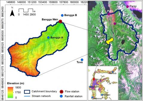
The baseline data for this study were collected from two rainfall and one streamflow gauging stations in the Bangga Catchment, one of the agricultural sub-basins in Sulawesi, Indonesia (Figure 1). Those two hydrologic instruments identified as Bangga A and Bangga B are located at GPS coordinates of 119°53'50"E and 01°16'55"S and 119°55'23"E and 01°14'25"S respectively. Meanwhile, the hydrometric instrument is geographically situated approximately 30 meters upstream of the Bangga Weir with coordinates of 119°55'10.31"E and 01°15'6.79"S. Data from the gauging stations for the period 2002-2014 were grouped into two types of data, daily rainfall and daily streamflow data.
The Bangga catchment is a part of the Palu River Basin with an area of around 68.19 km2 [34]. The catchment function is very important as it is the primary source of water supply and irrigation system in the middle and lower part of the catchment. Almost all residents who live in this catchment work as wetland and dry land farmers. The main commodities resulting from this agricultural practice are seasonal crops such as rice, corn, soybean, peanuts, and various types of vegetables, and long-lived crops such as cacao, coconut and hazelnut.
This catchment is a flood-prone area. Damage to the hydrometric instrument and flooding of residential and agricultural areas is one of the major impacts of flooding in the catchment. The flash flood in 2019 was the largest flood event ever to occur as a secondary impact of the 2018 Palu earthquake [32]. Debris flow triggered by the accumulation of heavy rainfall and landslides in the upper area, not only damages agricultural and residential areas but also causes a number of fatalities. Illustration of water disasters in this catchment requires emergency management at present and future program implementation.
Figure 1. Site of hydrologic and hydrometric gauges in the study area around the catchment as the main data source
2.2 Methods
The initial step of this study was carried out by selecting the average maximum daily rainfall data from the two rainfall gauges, as performed by Ahmad et al. [18]. A similar procedure was also applied to daily streamflow data. Two stages of rainfall data selection were applied. The first stage is selecting daily maximum rainfall data using the AMS approach and lastly is determining rainfall data based on peak over threshold (PDS). The selection of maximum daily streamflow data was also executed using the AMS method.
RDP, RDA and QDA were determined from selection of each data using frequency analysis. Four statistical distribution methods consisting of Normal, Normal Log, Pearson Log Type III and Gumbel were applied to perform the analysis. The general equation of the four distributions is given with the following formula [35]:
$x_{t}=\bar{\mu}+K_{t} \sigma$ (1)
where, $x_{t}$ = the magnitude of the T-year rainfall/streamflow event of such specified probability, $\bar{\mu}$ and $\sigma$ are the average and standard deviation of $x, K_{t}$ = frequency factor depending on the function of probability distribution and the recurrence interval of event. For Log Normal and Log Pearson Type III Distributions, $x_{t}, \mu$ and $\sigma$ are expressed in the logarithmic transformation. $K_{t}$ is obtained from the frequency factor table of each statistical distribution. However, several formulas have been developed to calculate $K_{t}$.
2.2.1 Normal distribution
$K_{t}$ is formulated as:.
$K_{t}=Z$ (2)
Z is the variate of standard normal distribution with unit standard deviation and a mean of zero. Z is equivalent to the following equation [36, 37]:
$Z=W-W^{\prime}$ (3a)
$W^{\prime}=\frac{2.515517+0.802853 W+0.010328 W^{2}}{1+1.432788 W+0.1892 .69 W^{2}+0.001308^{3}}$ (3b)
$W= \begin{cases}\sqrt{\ln \frac{1}{p},} & 0<p \leq 0.5 \\ \sqrt{1-p,} & \text { for others } p\end{cases}$ (4)
where, $p$ = probability exceedence which is equal to 1/T.
2.2.2 Log normal distribution
$K_{t}$ can be calculated similar to Z using Eq. (3) provided that all parameters are converted into a logarithmic transformation. However, if the transformation is not performed, $K_{t}$ can be predicted using the classical frequency factor:
$K_{t}=\left(\frac{1}{C_{v}}\right)\left\langle\exp \left[\begin{array}{c}
Z\left\{\ln \cdot\left(1+C_{v}^{2}\right)\right\}^{\frac{1}{2}} \\
-0.5\left\{\ln \left(1+C_{v}^{2}\right)\right\}
\end{array}\right]-1\right\rangle$ (5)
where, $C_{v}$ is coefficient of variance $\left(\frac{\sigma}{\mu}\right)$ of the normal distribution data. Using this $K_{t}$, then $x_{t}$ computation is carried out as in Normal distribution.
2.2.3 Log Pearson Type III distribution
There are some equations for calculating $K_{t}$ in this distribution such as Wilson-Hilferty approximation [38]. The equation was recommended for skewness coefficient $\left(C_{s}\right) \leq$ 2 and $0.01 \leq p \leq 0.99$.
$K_{t}=\left[\begin{array}{c}
Z+\left(Z^{2}-1\right) \frac{C_{s}}{6}+\frac{1}{3}\left(Z^{3}-6 Z\right)\left(\frac{C_{s}}{6}\right)^{2} \\
-\left(Z^{2}-1\right)\left(\frac{C_{s}}{6}\right)^{3}+Z\left(\frac{C_{s}}{6}\right)^{4}-\frac{1}{3}\left(\frac{C_{s}}{6}\right)^{5}
\end{array}\right]$ (6)
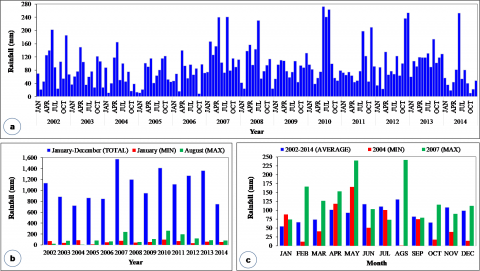
Figure 2. Characteristics of average rainfall at study sites in 2002-2014. (a). Monthly rainfall series, (b). Annual rainfall, minimum and maximum average of monthly rainfall respectively (January and August), and (c). Average monthly rainfall, annual minimum (2004) and annual maximum (2007)
2.2.4 Gumbell distribution
Onen and Bagatur [39] proposed an equation to estimate $K_{t}$ by substituting the reduced mean variable using regression analysis in original equation of Gumbel.
$K_{t}=\frac{-\ln \left\{\ln \left(\frac{T}{T-1}\right)\right\}-0.5775 n\left(-\frac{0.66}{n}\right)}{1.2811 n\left(-\frac{1.268}{n}\right)}$ (7)
where, n = the number of data.
The analysis in this work was performed using frequency analysis package named as AProb_4.1. The software was developed by Istiarto (2014) in the University of Gadjah Mada, Indonesia [40]. The package also involves other statistical tests such as the test of the significance of the distribution variable by evaluating the goodness of fit of the observed and predicted $x_{t}$. The two approaches used to assess it were Chi-square ($\chi^{2}$) and Kolmogorov–Smirnov (K-S) tests.
The final step of the study was to perform the relationship between RDP and RDA, RDA and QDA and RDP and QDA. The relationships of those variables were performed using linear regression analysis. Another more practical method is to use the trendline analytics tool in the spreadsheet program, and then the relationship between RDP and RDA as the final target of this work is solved analytically based on the RDP-RDA equation and RDA-QDA equations.
3.1 Rainfall and streamflow characteristics
The 13-year series of rainfall data at the study location indicates that the annual trend of average monthly rainfall intensity fluctuates annually with a range from 9.1 mm to 272.7 mm (Figure 2a). While the largest average annual rainfall was in 2007 and the lowest was in 2004 (Figure 2b). Accordingly, the minimum average monthly rainfall occurs in January and the maximum in August (Figure 2c). Rainfall patterns in this region are relatively similar to rainfall patterns in the tropics in general, although the rainfall peak shifts especially in the wet months. However, the annual rainfall in the range 722.2 mm and 1575.7 is lower than the average annual rainfall in the main catchment (Palu watershed) which reaches more than 2000 mm/year [32].
The rainfall pattern in the Bangga Catchment is also considered to represent the rainfall pattern in the Palu Watershed especially in the middle and downstream areas where the average annual rainfall for this region is below 1500 mm [32]. The rainfall characteristics in this area are influenced not only by the climatic conditions in the Palu Valley but also by the climate of the mountainous areas on the west and east sides of the Palu River. The great air pressure in the Palu Valley, originating from the movement of air from the Gulf of Palu and high solar radiation throughout the year also impacts the intensity and distribution of rainfall. These climatic factors also cause the daily evapotranspiration rate to be higher than the average daily rainfall. As a result of this condition, vegetation in the mountainous areas on the west and east sides of the Palu watershed has largely been degraded into open land.
Streamflow characteristics recorded at the gauging station in the period 2002-2014 also fluctuated throughout the year in proportion to the intensity of the channel. In the rainy season, streamflow increases and vice versa in the dry season, decreasing with relatively low variability. The indicator of the low variability of the streamflow is measured from the standard deviation of 2.5 m3/s. Within this time span, the streamflow fluctuates from 1.5 m3/s to 13.2 m3/s with an average of 4.6 m3/s. The relationship between monthly rainfall and average monthly discharge can be illustrated graphically as in Figure 3. It is seen as a linear relationship that is classified as a moderate correlation in the range of 0.60 to 0.70 [41, 42]. Several factors can influence the relationship between rainfall and streamflow correlations that are not so strong, especially the pattern of rainfall distribution and rainfall movement [5]. High intensity rain that is not evenly distributed in the entire catchment causes the accumulation of streamflow, which is not optimal, therefore, the correlation is low. In addition, high-intensity, fast moving rainfall also causes the same impact. The best solution to this problem is the availability of rainfall gauges which are installed evenly with high density in all catchment areas [43, 44].
Figure 3. A correlation graph of total monthly rainfall and average monthly streamflow in 2002-2014
3.2 Rainfall and streamflow data selection
The selection of rainfall and streamflow data as mentioned earlier is based on two approaches: AMS and ADS. The first approach is valid for both types of data, while the second approach is only applied to streamflow data. The results of data selection using both methods are presented in Table 1.
The reference for applying the AMS method is to select the maximum data for each year from the daily data. Using this method, a total of 13 rainfall and streamflow data have been selected respectively. The PDS approach is applied based on such threshold value. In the case of this study, threshold value is set at the smallest annual maximum of rainfall data. The number of selected data using this method is 74.
The selected rainfall data range based on the two approaches is 28.3 mm to 87.8 mm with an average of 55.83 mm for AMS and 43.26 mm for ADS. The variability of the data selected by the AMS method was slightly higher than the PDS approach with standard deviations of 16.88 mm and 12.99 mm, respectively. Meanwhile, the average streamflow data selected by the AMS method is 15.96 m3 /s in the range of 5.88 m3 /s to 15.96 m3/s and a standard deviation of 5.88 m3/s. Detailed observations from the results of the data selection illustrate that the three types of data have almost the same variability with each coefficient of variation: 30.23% (Rainfall-AMS), 29.81% (Rainfall-PDS) and 36.84 (Streamflow-AMS). The variability of the data shows that the level of uniformity of data is relatively high. Data uniformity is inversely proportional to data variability. However, the variability of the two data groups cannot be used as a reference to measure the correlation, except using covariance [45].
Table 1. Selected rainfall and flow data according to partial duration series and annual maximum series in the period 2002-2014
|
Year |
Rainfall (mm) |
AMS Streamflow Peak (m3/s) |
||||||||||||
|
AMS (mm) |
Partial Duration Series (PDS) with the Smallest Annual Maximum of Threshold |
Number of PDS Data |
||||||||||||
|
2002 |
72.0 |
28.3 |
50.4 |
52.5 |
63.5 |
64.6 |
72.0 |
|
|
|
|
|
6 |
9.11 |
|
2003 |
37.3 |
28.3 |
29.3 |
34.1 |
36.3 |
37.3 |
|
|
|
|
|
|
5 |
9.19 |
|
2004 |
46.4 |
33.5 |
34.9 |
39.4 |
46.4 |
|
|
|
|
|
|
|
4 |
9.02 |
|
2005 |
28.3 |
28.3 |
|
|
|
|
|
|
|
|
|
|
1 |
8.19 |
|
2006 |
44.9 |
31.2 |
33.5 |
36.1 |
39.1 |
44.9 |
|
|
|
|
|
|
5 |
7.14 |
|
2007 |
64.5 |
29.5 |
32.4 |
39.2 |
40.4 |
46.3 |
47.6 |
48.2 |
49.0 |
49.3 |
63.0 |
64.5 |
11 |
15.12 |
|
2008 |
65.0 |
32.7 |
32.9 |
37.8 |
65.0 |
|
|
|
|
|
|
|
4 |
15.96 |
|
2009 |
49.0 |
38.3 |
38.6 |
49.0 |
|
|
|
|
|
|
|
|
3 |
7.54 |
|
2010 |
78.0 |
31.9 |
34.8 |
42.1 |
48.3 |
53.4 |
63.3 |
78.0 |
|
|
|
|
7 |
15.45 |
|
2011 |
87.8 |
35.4 |
37.3 |
38.7 |
61.3 |
67.8 |
87.8 |
|
|
|
|
|
6 |
7.72 |
|
2012 |
45.3 |
30.2 |
36.0 |
38.0 |
38.1 |
38.4 |
45.2 |
45.3 |
|
|
|
|
7 |
6.40 |
|
2013 |
55.7 |
29.6 |
30.5 |
30.7 |
31.7 |
33.4 |
34.2 |
35.8 |
39.0 |
40.6 |
50.6 |
55.7 |
11 |
15.18 |
|
2014 |
51.6 |
28.8 |
42.9 |
47.1 |
51.6 |
|
|
|
|
|
|
|
4 |
5.88 |
3.3 Frequency analysis
As previously conveyed, frequency analysis of selected rainfall and streamflow data was performed using four statistical distributions: Normal, Log Normal, Log Pearson Type III and Gumbel. The application of two types of variable significance tests on the four distribution methods shows that the only distribution rejected by both Chi-square and Kolmogorov-Smirnov tests is the Normal distribution. Some researchers such as Brotowiryatmo [5] and Estiningrum et al. [46] have proven that rainfall and streamflow events in Indonesia rarely follow the normal distribution. In general, extreme data covering all hydrological data are relatively very seldom suited to the normal distribution. However, some cases of rainfall and streamflow data may follow Normal distribution [5].
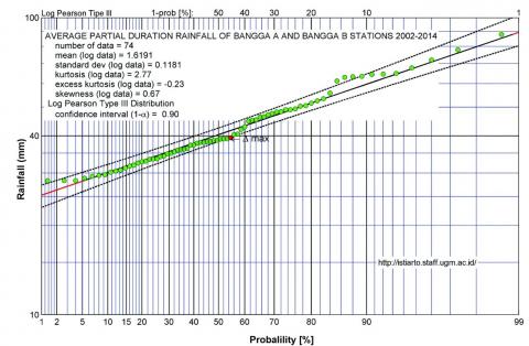
Table 2 presents the results of testing the significance of variables on the four statistical distributions. Three distribution methods except Normal meet the statistical distribution test requirements with values of $\chi^{2}$) and $\Delta$ less than the critical value. Log Pearson Type III was selected as the best distribution with the highest difference of $\chi^{2}$) and $\Delta$. The significance of this distribution can also be illustrated by plotting position as shown in Figure 4 for the PDS rainfall data.
The frequency of analysis of the three types of data results in a design magnitude with such recurrence intervals denoted as RDP, RDA and QDA as presented in Table 3. This recurrence interval is related to the event probability of the parameter representing the variable. In hydrology, this is directly associated with the costs and risks of an area protection program from flood hazards [47]. The increase in recurrence interval is proportional to the risk reduction and the increase in the cost of the program [48]. These two factors become the basis for consideration in setting recurrence intervals so that a structure with higher reliability and lower cost will be obtained.
Figure 4. A Log Pearson Type III probability plot of partial duration rainfall data for performing statistical distribution tests, generated using AProb_4.1 [40]
Table 2. Statistical test on the four distribution methods of 74 selected rainfall data
|
Statistical Distribution |
Statistical Test |
|||||||
|
Chi-square |
Kolmogorov- Smirnov |
|||||||
|
$\chi$2comp |
$\chi$2crit |
Difference |
Remark |
$\Delta_{\max }$ |
$\Delta$crit |
Difference |
Remark |
|
|
Normal |
15.32 |
5.99 |
- |
Rejected |
0.16 |
0.16 |
- |
Rejected |
|
Log Normal |
5.87 |
5.99 |
0.13 |
Accepted |
0.13 |
0.16 |
0.03 |
Accepted |
|
Log Pearson Type III |
0.19 |
5.99 |
5.80 |
Accepted |
0.08 |
0.16 |
0.07 |
Accepted |
|
Gumbel |
3.16 |
3.84 |
0.68 |
Accepted |
0.10 |
0.16 |
0.05 |
Accepted |
Table 3. Design rainfall and flow computed from PDS and AMS data using frequency analysis
|
Parameters |
Recurrence Interval (year) |
|||||||
|
1.1 |
2 |
5 |
10 |
20 |
50 |
100 |
1000 |
|
|
RDP (mm) |
30.12 |
40.37 |
51.58 |
59.72 |
68.07 |
79.78 |
89.29 |
126.23 |
|
RDA (mm) |
35.45 |
54.32 |
69.75 |
78.77 |
86.68 |
96.08 |
102.62 |
122.00 |
|
QDA (m3/s) |
7.05 |
9.82 |
12.97 |
15.31 |
17.76 |
21.27 |
24.17 |
35.81 |
It can be observed in Table 3 that all RDP values are smaller than RDA values at the corresponding recurrence interval. This relates to the maximum amount of data selected. The rainfall data selected by the AMS and PDS methods indicate that the average PDS rainfall is almost equivalent to 75% of the average AMS rainfall. In other words, the average PDS rainfall is smaller than the average AMS rainfall. In Eq. (1), this mean value is the main factor in determining the RDP, RDA and QDA in addition to the standard deviations from the data. Accommodating a certain number of values below the maximum value will have an impact on the decrease in the average value. This has also been proven by many researchers that the determination of the peak over threshold in the PDS method affects the number of selected data and the average value and finally it produces an estimated RDP that is always lower than the RDA [20, 21, 23, 26, 49].
3.4 Peak flood formula
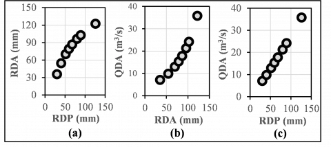
The ultimate goal of this study is to formulate a streamflow equation based on selected PDS rainfall data. This equation is a representation of the flood peak equation with such a recurrence interval. Early indications of the relationship between these variables show different trends. The relationship between RDP and RDA is illustrated as a logarithmic function (Figure 5a), while the relationship between RDA-QDA and EDP-QDA are represented as exponential and power functions respectively (Figure 5b and Figure 5c). The three functions that represent the relationships between those variables are very high levels of strength with a correlation coefficient close to 1. The trend of the relationship between these variables may change depending on the characteristics of the selected data. Another data is needed as a comparison to prove that various types of functions might be able to present the relation.
Figure 5. Nonlinear relationships between selected data. (a). RDP vs. RDA (logarithmic function), (b). RDA vs. QDA (exponential function), and (c). RDP vs. QDA (power function)
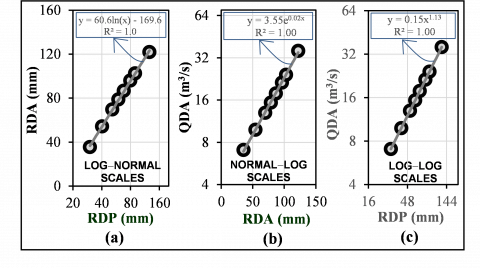
Figure 6. Logarithmic transformation of data to form linear relationships. (a). Logarithmic-Normal scales, (b). Normal-Logarithmic scale, and (c). Logarithmic-Logarithmic scales
Figure 7. Performance representation of predicted design rainfall and flow. (a). Design rainfall computed using Eq. 11 (RDA1) and frequency analysis (RDA2), and (b). Design flow computed using Eq. 16 (QDA1) and frequency analysis (QDA2)
A very interesting thing to observe is that none of the relationships between variables shows a linear function. To make a statistical formulation based on linear regression, one or two of the variables must be converted into a logarithmic transformation. The results of the transformation are shown in Figure 6 in the form of Log-Normal scale, Normal-Log scale and Log-Log scale.
Linear regression is performed to compile the formulas of each function using R software. The equation produced from this regression analysis is as follows:
$R D A=60.5538 \ln R D P-169.5743$ (8)
$\ln Q D A=0.0087 R D A+1.2678$ (9)
$0.8816 \ln Q D A=\ln R D P+1.6839$ (10)
When using the add trendline tool in a spreadsheet program, the equation can be stated as:
$R D A=60.5538 \ln R D P-169.5743$ (11)
$Q D A=3.5532 \exp (0.0187 R D A)$ (12)
$Q D A=0.1481 R D P^{1.1343}$ (13)
Now focus on Eq. (9) to formulate the final equation of QDA as a function of RDP. Simplification of Eq. (9) to Eq. (12) can be done analytically. Applying e to left and right side of Eq. (9) produces:
$Q D A=3.5532 \exp (0.0187 R D A)$ (14)
$Q D A=\exp (0.0187 R D A) \exp (1.2678)$ (15)
$Q D A=3.5532 \exp (0.0187 R D A)$ (16)
Eq. (16) is the same as Eq. (12). Similar analytic methods can also be applied to formulate the Eq. (11) and Eq. (13) from Eq. (8) and Eq. (10). To obtain the final formula between RDA and QDA, RDA in Eq. (16) is substituted by the RDA in Eq. (11) as follows:
Table 4. Absolute error of predicted flow based on RDP data
|
QDA1 (m3/s) |
QDA2 (m3/s) |
Absolute Error |
|
7.05 |
7.05 |
0.00064 |
|
9.82 |
9.82 |
0.00419 |
|
12.97 |
12.97 |
0.00135 |
|
15.31 |
15.31 |
0.00122 |
|
17.76 |
17.76 |
0.00109 |
|
21.27 |
21.26 |
0.01127 |
|
24.17 |
24.15 |
0.01758 |
|
35.81 |
35.76 |
0.05404 |
|
Mean Absolute Error (MAE) |
0.01142 |
|
|
Correlation coefficient (r) |
0.9988 |
|
Eq. (20) is the final equation of the targeted formula. This formula shows very good performance with a very low average Mean Absolute Error (MAE) [50] and a very high correlation coefficient (Figure 7 and Table 4). Therefore, this equation can be applied to sub-catchments throughout the study area and beyond.
The limitations of hydrologic data especially rainfall and streamflow data have become a serious issue for researchers to perform an analysis in the field of water resource management. This data limitation relates to the unavailability of measuring instruments installed in an area or the inability of measurement instruments to present data of sufficient quantity and quality. A partial duration series (PDS) approach has been developed to overcome this problem to increase the number of data from short data series. This PDS approach has been adopted in this study for flood estimation in an agricultural catchment.
This work successfully developed an equation expressing the relationship between design flood (QDA) generated from the annual maximum series (AMS) of daily streamflow data and design rainfall (RDP) predicted from PDS of daily rainfall data. QDA and RDA are the two main variables of the equation that are formulated using frequency analysis based on selected statistical distribution of Log Pearson Type III. The formula declared with the power equation shows very high performance with a very low Mean Absolute Error (MAE) and a very strong correlation coefficient (r). This equation is recommended for application in all outlets of the sub-catchments in the entire catchment of the study area
The authors gratefully acknowledge the Indonesian Ministry of Education, Culture, Research and Technology for supporting this work through Fundamental Research Grant (No: 155/E4.1/AK.04.PT/2021).
|
AMS |
annual maximum series |
|
Cv |
coefficient of variance |
|
PDS |
partial duration series |
|
RDA |
annual maximum series of rainfall |
|
RDP |
partial duration series of rainfall |
|
QDA |
annual maximum series of discharge |
|
Kt |
frequency factor |
|
p |
probability exceedance which is equal to 1/T |
|
xt |
the magnitude of the T-year rainfall/streamflow event of such specified probability, mm, m3. s-1 |
|
Z |
the variate of standard normal distribution with unit standard deviation and a mean of zero |
|
Greek symbols |
|
|
$\Delta$ |
Kolmogorov–Smirnov tests parameter |
|
$\sigma$ |
standard deviation of x, |
|
$\bar{\mu}$ |
the average of x, |
|
$\chi$2 |
Chi-squared tests parameter |
|
Subscripts |
|
|
t |
Time, h |
[1] Yeh, H., Chen, Y., Wei, C., Chen, R. (2011). Entropy and kriging approach to rainfall network design. Journal of Paddy and Water Environment, 9: 343-355. https://doi.org/10.1007/s10333-010-0247-x
[2] Canchala-Nastar, T., Carvajal-Escobar, Y., Alfonso-Morales, W., Cerón, W.L., Caicedo, E. (2019). Estimation of missing data of monthly rainfall in southwestern Colombia using artificial neural networks. Data in Brief, 26: 104517. https://doi.org/10.1016/j.dib.2019.104517
[3] Bayat, B., Hosseini, K., Nasseri, M., Karami, H. (2019). Challenge of rainfall network design considering spatial versus spatiotemporal variations. Journal of Hydrology, 574: 990-1002. https://doi.org/10.1016/j.jhydrol.2019.04.091
[4] Nyssen, J., Vandenreyken, H., Poesen, J., Moeyersons, J., Deckers, J., Haile, M., Salles, C., Govers, G. (2005) Rainfall erosivity and variability in the Northern Ethiopian Highlands. Journal of Hydrology, 311: 172-187. https://doi.org/10.1016/j.jhydrol.2004.12.016
[5] Brotowiryatmo, S.H. (2008). Hydrology: Theory, Problems and Solving. Nafiri Offset, Yogyakarta. [in Indonesian].
[6] Boulomytis, V.T.G., Zuffo, A.C., Imteaz, M.A. (2018). Derivation of design rainfall and disaggregation process of areas with limited data and extreme climatic variability. International Journal of Environmental Research, 12: 147-166. https://doi.org/10.1007/s41742-018-0079-x
[7] Wang, L.-P., Ochoa-Rodriguez, S., Willems, P., Onof, C. (2014). Improving the applicability of gauge-based radar rainfall adjustment methods to urban pluvial flood modelling and forecasting using local singularity analysis. Proc. 2nd Int. Symposium on Weather Radar and Hydrology, Davis, pp. 1-10.
[8] Beskow, S., Caldeira, T.L., de Mello, C.R., Faria, L.C., Guedes, H.A.S. Multiparameter probability distributions for heavy rainfall modeling in extreme southern Brazil. Journal of Hydrology: Regional Studies, 4: 123-133. https://doi.org/10.1016/j.ejrh.2015.06.007
[9] Marra, F., Nikolopoulos, E.I., Anagnostou, E.N., Morina, E. (2018). Metastatistical extreme value analysis of hourly rainfall from short recoRDP: Estimation of high quantiles and impact of measurement errors. Advances in Water Resources, 117: 27-39. https://doi.org/10.1016/j.advwatres.2018.05.001
[10] Guru, N., Jha, R. (2016). Flood estimation in Mahanadi river system, India using partial duration series. Georisk: Assessment and Management of Risk for Engineered Systems and Geohazard, 10(2): 135-145. https://doi.org/10.1080/17499518.2015.1116013
[11] Ntegeka, V., Willems, P. (2008). Trends and multidecadal oscillations in rainfall extremes, based on a more than 100-year time series of 10 min rainfall intensities at Uccle, Belgium. Water Resources Research, 44(7): W07402. https://doi.org/10.1080/17499518.2015.1116013
[12] Vandenberghe, S., Verhoest, N.E.C., Onof, C., Baets, D.B. (2011). A comparative copula‐based bivariate frequency analysis of observed and simulated storm events: A case study on Bartlett‐Lewis modeled rainfall. Water Resources Research, 47(7): W07529. https://doi.org/10.1029/2009WR008388
[13] Gao, Z., Long, D., Tang, G., Zeng, C., Huang, J., Hong, Y. (2017). Assessing the potential of satellite-based precipitation estimates for flood frequency analysis in ungauged or poorly gauged tributaries of China’s Yangtze River basin. Journal of Hydrology, 550: 478-496. https://doi.org/10.1016/j.jhydrol.2017.05.025
[14] Młyński, D., Petroselli, A., Walega, A. (2018). Flood frequency analysis by an event-based rainfall-runoff model in selected catchments of southern Poland. Soil & Water Research, 13(3): 170-176. https://doi.org/10.17221/153/2017-SWR
[15] Adamiak, E.B., Licznar, P., Zaleski, J. (2019). Criteria for identifying maximum rainfall determined by the peaks-over-threshold (POT) method under the Polish Atlas of Rainfall Intensities (PANDa) project. Meteorology Hydrology and Water Management, 7(1): 3-12. https://doi.org/10.26491/mhwm/93595
[16] Kazemikia, S., Besharati, T., Zolfaghari, M., Ghanbarpour, M.R. (2016) Comparative study of maximum and partial duration series in flood frequency analysis (Case study in Talar and Babolrud watersheds in Mazandaran Province). Iranian Journal of Watershed Management Science and Engineering, 10(34): 113-117. https://doi.org/10.1016/0022-1694(73)90051-6
[17] Agilan, V., Umamahesh, N.V. (2017). Non-stationary rainfall intensity-duration-frequency relationship: A comparison between annual maximum and partial duration series. Water Resources Management, 31: 1825-1841. https://doi.org/10.1007/s11269-017-1614-9
[18] Ahmad, I., Khan, D.A., Almanjahie, I.M., Chikr-Elmezouar, Z., Laksaci, A. (2019). At-site rainfall frequency analysis using partial duration series and annual maximum series: A case study. Applied Ecology and Environmental Research, 17(4): 8351-8367. https://doi.org/10.15666/aeer/1704_83518367
[19] Soto, J., Palenzuela, J.A., Galve, J.P., Luque, J.A., Azañón, J.M., Tamay, J., Irigaray, C., (2019). Estimation of empirical rainfall thresholds for landslide triggering using partial duration series and their relation with climatic cycles. An application in southern Ecuador. Bulletin of Engineering Geology and the Environment, 78: 1971-1987. https://doi.org/10.1007/s10064-017-1216-z
[20] Madsen, H. (1997). Comparison of annual maximum series and partial duration series methods for modeling extreme hydrologic events. Water Resources Research, 33(4): 747-757. https://doi.org/10.1029/96WR03848
[21] Bezak, N., Brillya, M., Šraj, M. (2014). Comparison between the peaks over threshold method and the annual maximum method for flood frequency analyses. Hydrological Sciences Journal, 59(5): 959-977. https://doi.org/10.1080/02626667.2013.831174
[22] Zin, W.Z.W., Shinyie, W.L., Jemain, A.A. (2015). Modelling of extreme rainfall events in peninsular Malaysia based on annual maximum and partial duration series. AIP Conference Proceedings, 164: 312-320. https://doi.org/10.1063/1.4907461
[23] Chang, K.B., Lai, S.H., Othman, F. (2016). Comparison of annual maximum and partial duration series for derivation of rainfall intensity-duration-frequency relationships in Peninsular Malaysia. Journal of Hydrologic Engineering, 21(1): 1943-5584. https://doi.org/10.1061/(ASCE)HE.1943-5584.0001262
[24] Gado, T.A., Nguyen, V.T.V. (2016). Regional estimation of floods for ungauged sites using partial duration series and scaling approach. Journal of Hydrologic Engineering, 21(12): 1943-5584. https://doi.org/10.1061/(ASCE)HE.1943-5584.0001439
[25] Karim, F., Hasan, M., Marvanek, S. (2017). Evaluating annual maximum and partial duration series for estimating frequency of small magnitude floods. Water, 9: 481. https://doi.org/10.3390/w9070481
[26] Campenhout, J.V., Houbrechts, G., Peeter, A, Petit, F. (2020). Return period of characteristic discharges from the comparison between partial duration and annual series, application to the Walloon rivers (Belgium). Water, 12: 792. https://doi.org/10.3390/w12030792
[27] Gregersen, I.B. (2017). A regional and nonstationary model for partial duration series of extreme rainfall. Water Resources Research, 53(4): 2659-2678. https://doi.org/10.1002/2016WR019554
[28] Haddad, K., Rahman, A. (2014). Derivation of short-duration design rainfalls using daily rainfall statistics. Natural Hazards, 74: 1391-1401. https://doi.org/10.1007/s11069-014-1248-7
[29] Guru, N., Jha, R. (2020). Application of soft computing techniques for river flow prediction in the downstream catchment of Mahanadi river basin using partial duration series, India. Iranian Journal of Science and Technology, 44: 279-297. https://doi.org/10.1007/s40996-019-00272-0
[30] Kamal, V., Mukherjee, S., Singh, P., Sen, R., Vishwakarma, C.A., Sajadi, P., Asthana, H., Rena, V. (2017). Flood frequency analysis of Ganga river at Haridwar and Garhmukteshwar. Applied Water Science, 7: 1979-1986. https://doi.org/10.1007/s13201-016-0378-3
[31] Hajani, E., Rahman, A. (2018). Design rainfall estimation: Comparison between GEV and LP3 distributions and at-site and regional estimates. Natural Hazards, 93: 67-88. https://doi.org/10.1007/s11069-018-3289-9
[32] Tunas, I.G., Tanga, A., Oktavia, S.R. (2020). Impact of landslides induced by the 2018 Palu earthquake on flash flood in Bangga river basin, Sulawesi, Indonesia. Journal of Ecological Engineering, 21(2): 190-200. https://doi.org/10.12911/22998993/116325
[33] Tunas, I.G., Maadji, R. (2018). The use of GIS and hydrodynamic model for performance evaluation of flood control structure. International Journal on Advanced Science Engineering and Information Technology, 8(6): 2413-2420. https://doi.org/10.18517/ijaseit.8.6.7489
[34] Tunas, I.G., Anwar, N., Lasminto, U. (2019). A synthetic unit hydrograph model based on fractal characteristics of watersheds. International Journal of River Basin Management, 17(4): 465-477. https://doi.org/10.1080/15715124.2018.1505732
[35] Chow, V.T., Maidment, D., Mays, L. (1951). Applied Hydrology. McGraw-Hill Book Company, New York.
[36] Bhakar, S.R., Bansal, A.K., Chhajed, N., Purohit, R.C. (2006). Frequency analysis of consecutive days maximum rainfall at Banswara, Rajasthan, India. ARPN Journal of Engineering and Applied Sciences, 1(3): 64-67.
[37] Deraman, W.H.A.W., Mutalib, N.J.A.M., Mukhtar, N.Z. (2017). Determination of return period for flood frequency analysis using normal and related distributions. IOP Conference Series: Journal of Physics, 890: 012162. https://doi.org/10.1088/1742-6596/890/ 1/012162
[38] Chowdhury, J.U., Stedinger, J.R., Confidence interval for design floods with estimated skew coefficient. Journal of Hydraulic Engineering, 117(7): 811-831. https://doi.org/10.1061/(ASCE)0733-9429(1991)117:7(811)
[39] Onen, F., Bagatur, T. (2017). Prediction of flood frequency factor for Gumbel distribution using regression and GEP model. Arabian Journal for Science & Engineering, 42: 3895-3906. https://doi.org/10.1007/s13369-017-2507-1
[40] Istiarto. (2021). Frequency analysis of hydrology data (AProb_4.1). https://istiarto.staff.ugm.ac.id/index.php/ 2014/12/analisis-frekuensi-data-hidrologi-aprob_4-1/, 2014, Accessed on June 17th, 2021.
[41] Akoglu, H. (2018). User's guide to correlation coefficients. Turkish Journal of Emergency Medicine, 18(3): 91-93. https://doi.org/10.1016/j.tjem.2018.08.001
[42] Aoun, N., Bouchouicha, K. (2017). Simple correlation models for estimation of horizontal global solar radiation for Oran, Northwest Algeria. International Journal of Engineering Research in Africa, 32: 124-132. https://doi.org/10.4028/www.scientific.net/JERA.32.124
[43] Nikolopoulos, E.I., Borga, M., Creutin, J.D., Marra, F. (2015). Estimation of debris flow triggering rainfall: Influence of rain gauge density and interpolation methods. Geomorphology, 243: 40-50. https://doi.org/10.1016/j.geomorph.2015.04.028
[44] Tan, M.L., Yang, X. (2020). Effect of rainfall station density, distribution and missing values on SWAT outputs in tropical region. Journal of Hydrology, 584: 124660. https://doi.org/10.1016/j.jhydrol.2020.124660
[45] Sands, D.E. (1997). Correlation and covariance. Journal of Chemical Education, 54: 90-94. https://doi.org/10.1021/ ed054p90
[46] Estiningrum, T., Rusgiyono, A., Wilandari, Y. (2015). Application of peak over threshold using the Generalized Pareto Distribution (GPD) approach and Moment-L parameter estimation on rainfall data. Journal Gaussian, 4: 141-150. https://doi.org/10.14710/j.gauss.v4i1.8154
[47] Read, L.K., Vogel, R.M. (2015). Reliability, return periods, and risk under nonstationarity. Water Resources Research, 51(8): 638-6398. https://doi.org/10.1002/2015WR017089
[48] Olsen, A.S., Zhou, Q., Linde, J.J., Arnbjerg-Nielsen, K. (2015). Comparing methods of calculating expected annual damage in urban pluvial flood risk assessments. Water, 7: 255-270. https://doi.org/10.3390/w7010255
[49] Srikanthan, S. (2014). A comparison of annual maximum and partial duration series in frequency analysis. Proc. Hydrol. Water Resour. Sympo, Engineers Australia’s National Committee on Water Engineering, pp. 374-381. https://doi.org/10.1061/(ASCE)HE.1943-5584.0001262
[50] Odeyemi, S.O., Akinpelu, M.A., Abdulwahab, R., Dauda, K.A., Chris-Ukaegbu, S. (2020). Scour depth prediction for Asa Dam Bridge, Ilorin, using artificial neural network. International Journal of Engineering Research in Africa, 47: 53-62. https://doi.org/10.4028/www.scientific.net/JERA.47.53