Nuttibase Charupeng* | Prapot Kunthong
© 2022 IIETA. This article is published by IIETA and is licensed under the CC BY 4.0 license (http://creativecommons.org/licenses/by/4.0/).
OPEN ACCESS
Moisture-induced swelling, or hygroexpansion, has been known to greatly deteriorate the durability of wood fiber-polymer composites (WPC). It is generally very expensive to perform experiments to completely obtain the diffusion kinetics as the process occurs in a very extended period of time. For the first time, we have developed a space-time finite element algorithm that employs time discontinuous Galerkin (TDG) method for time-dependent 3D hygro-mechanical behaviours of WPC. The formulation of matrix equations in spatial and temporal domains are explained in detail. A block Gauss-Seidel iterative method is used in the predictor/multi-corrector multi-pass algorithm, which efficiently yields unconditionally stable and high-order accurate solutions. The model is validated by comparing the predicted time-dependent hygroexpansion with that obtained in a previous experimental study. The quantitative analysis ensures the reliability of model, based on a Fickian diffusion process. With our adaptive time-stepping scheme that bases on the embedded solution from the multi-pass iterations, the model efficiently progresses the kinetics with relatively large time steps. A runtime of a few hours compared to about three months of actual laboratory experimentation confirms the novelty and robustness of our model.
space-time finite element method, time-discontinuous Galerkin, hygro-mechanical modeling, wood fiber-polymer composites
As is well known, wood fiber reinforced composites have been used in the building materials industry for several decades due to their low cost, light weight, biodegradability, abrasion resistance, and good specific properties. However, moisture-induced expansion, i.e., hygroexpansion, is one of the major drawbacks of wood-based composites. Unlike wood fibers, matrix components in wood-based composites, such as polymers, are much less susceptible to water absorption than wood [1-3]. The drastic difference in hygroelastic properties can even lead to serious problems in the case of wood fiber-polymer composites (WPC), such as buckling and warping of the installed WPC panels [4]. Therefore, studying the hygro-mechanical behaviours of WPC is an essential part of improving the durability of the materials.
It has been shown experimentally [5-8] that the diffusion kinetics of water in WPC takes place over a very long period of time - from weeks to a few months, depending on the diffusivity of the materials. Therefore, laboratory experiments are sometimes too expensive to obtain fully meaningful results. Consequently, hygro-mechanical modeling is becoming increasingly important. Numerous hygro-mechanical modeling studies are conducted for wood-based materials [9-12] and for polymeric materials [13-15], but there is very little research on predicting the time-dependent hygro-mechanical behaviours of WPC. There is particularly little research that attempts to accurately predict the three-dimensional anisotropic responses of WPC subjected to water absorption.
Mbacké et al. [16] have used a numerical method to study the hygro-mechanical behaviours of homogenised composites, determining the time-dependent mechanical properties as a function of the moisture content of the materials. However, the model ignores the complexity of the anisotropy of materials and uses simple linear interpolation to obtain the resulting properties, leading to inaccurate predictions in the case of WPC. In another study [17], a multi-scale analytical model for stress-dependent moisture diffusion in fiber-reinforced polymer matrix composites was proposed under the assumption that the fibers do not absorb moisture. Thus, it is not applicable to the case of WPC where both constituents respond to moisture transport to different extents.
The finite element method (FEM) has been used extensively in the modeling and analysis of a composite structure with randomly distributed short fiber reinforced composites [18, 19]. Time-dependent problems are usually solved using FEM by first discretising the spatial domain and solving the resulting ordinary differential equation in discrete time steps. This method is commonly known as semi-discretisation. Like heat transfer problems, moisture diffusion in materials can be considered as a first-order parabolic problem, and perhaps the most commonly used methods for time integration are classified as single-step/single-solver methods (SS/SS) [20]. Such methods are based on solving a system of $n_{e q}$ linear equations leading to second-order accuracy by unconditionally stable implicit SS/SS methods such as the trapezoidal method.
However, in applications where time is greatly extended, the SS/SS methods can lead to an accumulation of errors when using large time steps. The most efficient way to solve the above problems is to discretise the temporal domain with an accuracy no less than that of the spatial domain. This is also known as space-time finite element method, which was developed by Hughes and Hulbert [21]. The method is based on the time-discontinuous Galerkin finite element method (TDG-FEM), which is possibly considered one of the best methods for time integration in a discretised temporal domain. It provides relatively high accuracy with good stability. Due to the large linear space-time linear systems of equations and the relatively high computational cost of solving non-symmetric TDG matrices directly, several techniques [22-24] have been developed. As a result, there are now several applications of TDG-FEM [25-28] However, to our knowledge, there are no studies using TDG-FEM to investigate the hygro-mechanical behaviours of WPC.
The current study has two objectives: 1) to develop a complete and efficient TDG-FEM algorithm written in MATLAB for hygro-mechanical behaviours of WPC and 2) to validate the model by comparing the solutions with corresponding experiments, investigating and discussing the reliability with respect to Fick’s theory.
The present paper is organised as follows. First, the formulation of the TDG-FEM matrix equations in space and time for the hygro-mechanical behaviours of WPC is presented. Then, the predictor/multi-corrector is described using a multi-pass algorithm from [24] and applied to the first-order parabolic moisture diffusion problem. A suitable adaptive time-stepping scheme is briefly explained. Then, the overall algorithm with the necessary defined material parameters is used to calculate the moisture evolution and the resulting hygroexpansion of the composites. The convergence of the mesh is considered. The efficiency of the time-stepping scheme using the embedded solution approach is discussed. It is followed by model validation and quantitative analysis of model reliability.
The general diffusion equation of moisture in a given material according to Fick’s second law reads:
$\frac{\partial W}{\partial H} \frac{\partial H}{\partial t}=\nabla \cdot\left(D_{h} \nabla H\right)$ (1)
where, ∂W/∂H is the moisture capacity that can be obtained through the equilibrium adsorption isotherm of the material, H represents the relative humidity ranging from zero to one, ∇H denotes the gradient vector of humidity. Also, Dh is the diffusion coefficient of moisture in the material or moisture diffusivity in m2/s. In a 3D Cartesian system or X space:
$D_{h}=\left[\begin{array}{lll}D_{h, x} & 0 & 0 \\ 0 & D_{h, y} & 0 \\ 0 & 0 & D_{h, z}\end{array}\right]$ (2)
where, Dh,x, Dh,y and Dh,z are the diffusion coefficients in the respective directions, which are are assumed to be constant. Therefore, Eq. (1) can be re-written for the 3D diffusion equation as:
$\frac{\partial H}{\partial t}=\frac{1}{\partial W / \partial H}\left(D_{h, x} \frac{\partial^{2} H}{\partial x^{2}}+D_{h, y} \frac{\partial^{2} H}{\partial y^{2}}+D_{h, z} \frac{\partial^{2} H}{\partial z^{2}}\right)$ (3)
The moisture absorption gives rise to hygroexpansion of material via:
$\boldsymbol{\varepsilon}_{h}=\left\{\begin{array}{l}\varepsilon_{h, x} \\ \varepsilon_{h, y} \\ \varepsilon_{h, z} \\ 0 \\ 0 \\ 0\end{array}\right\}=\Delta H\left\{\begin{array}{l}\beta_{x} \\ \beta_{y} \\ \beta_{z} \\ 0 \\ 0 \\ 0\end{array}\right\}$ (4)
where, ΔH is the change in humidity content, and βx, βy and βz are the directional hygroexpansion coefficients of material. The hygroexpansion strains do not contribute to shear deformation, leading to zero shear strains in Eq. (4). Consequently, the hygroelastic stress-strain relationships in X of the total strain, ε, elastic strains, εm can, therefore, be written as:
$\sigma=D_{m} \varepsilon_{m}=D_{m}\left(\varepsilon-\varepsilon_{h}\right)$ (5)
where,
$\sigma={ }^{T}\left\{\begin{array}{llllll}\sigma_{x} & \sigma_{y} & \sigma_{z} & \tau_{x y} & \tau_{y z} & \left.\tau_{z x}\right\}\end{array}\right.$ (6)
and
$\varepsilon_{m}={ }^{T}\left\{\frac{\partial u}{\partial x}, \frac{\partial v}{\partial y}, \frac{\partial w}{\partial z}, \frac{\partial v}{\partial z}+\frac{\partial w}{\partial y}, \frac{\partial w}{\partial x}+\frac{\partial u}{\partial z}, \frac{\partial u}{\partial y}+\frac{\partial v}{\partial x}\right\}$ (7)
The symbol T denotes transpose operation, σ denotes normal stresses, τ denotes shear stresses, u, v and w are the components of strain in x, y and z respectively, Dm is defined as:
$D_{m}$
$=\left[\begin{array}{llllll}1 / E_{x} & -v_{x y} / E_{x} & -v_{x z} / E_{x} & 0 & 0 & 0 \\ -v_{y x} / E_{y} & 1 / E_{y} & -v_{y z} / E_{y} & 0 & 0 & 0 \\ -v_{z x} / E_{z} & -v_{z y} / E_{z} & 1 / E_{z} & 0 & 0 & 0 \\ 0 & 0 & 0 & 1 / G_{y z} & 0 & 0 \\ 0 & 0 & 0 & 0 & 1 / G_{z x} & 0 \\ 0 & 0 & 0 & 0 & 0 & 1 / G_{x y},\end{array}\right]^{-1}$ (8)
where, E’s and G’s are elastic and shear moduli. v’s are Poisson’s ratios.
The equilibrium equations of a differential volume element that are satisfied over the physical domain are given in a tensor notation as:
$\sigma_{i j, j}+f_{i}=0$ (9)
where, σij are the stress components in the Cartesian stress tensor, fi is the component of the body force vector along the i direction, and j represents partial differentiation with respect to the j coordinate. Respectively, the essential and natural boundary conditions are:
$u_{i}(X)=\bar{u}_{i}$; on $\Gamma_{u}$ (10)
$\sigma_{i j} \hat{n}_{j}=\bar{t}_{i} ;$ on $\Gamma_{t}$ (11)
where, $u_{i}(X)$ is the displacement along the i direction of the point at coordinates X, $\bar{u}_{i}$ is the corresponding specified boundary displacement at the point, $\hat{n}_{j}$ is the component of unit normal vector in the j direction, and $\bar{t}_{i}$ is the specified boundary stress along the i direction.
Therefore, the governing equations of three-dimensional hygro-mechanical behaviours in a matrix form can be obtained by substituting the corresponding stress components from Eq. (6) into that of Eq. (9).
There is no or very little commercial software capable of modeling such a time-dependent moisture diffusion problem using high-accuracy adaptive time integration methods. Therefore, to simulate the hygro-mechanical behaviours of WPC, we have developed a complete algorithm written in MATLAB [29]. With the following series of FE formulations in space and time, the overall algorithmic structure is summarised in Figure 1.
Figure 1. Overall FE-based algorithm. ← and → denote input and output respectively
3.1 3D FE formulation in spatial domain
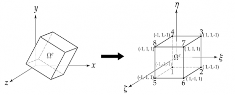
For each element in space, i.e. Ωe, an eight-node hexahedron with natural coordinates Ξ as shown in Figure 2 is used. Trilinear Lagrange interpolation functions (ξj, ηj, ζj) of local node j are applied:
$\Psi_{j}^{e}(\Xi)=\frac{1}{8}\left(1+\xi \xi_{j}\right)\left(1+\eta \eta_{j}\right)\left(1+\zeta \zeta_{j}\right)$ (12)
The element displacements, i.e., Ue=T{ue ve we}, are interpolated in terms of the shape functions in Eq. (12) and nodal displacements $u_{j}^{e}, v_{j}^{e}$ and $w_{j}^{e}$ as:
$u^{e}=\sum_{j=1}^{8} \Psi_{j}^{e} u_{j}^{e}, v^{e}=\sum_{j=1}^{8} \Psi_{j}^{e} v_{j}^{e}, w^{e}=$$\sum_{j=1}^{8} \Psi_{j}^{e} w_{j}^{e}$ (13)
The values of H are also interpolated from the nodes, in which semi-discretisation is used. The approximated humidity over Ωe is as follows:
$H^{e}(X, t)=\Psi^{e}(X) H^{e}(t)$ (14)
where, He(t) contains the nodal humidity values at time t. The first order time derivative of Eq. (14) is, therefore, obtained as:
$\frac{\partial}{\partial t} H^{e}(X, t)=\Psi^{e}(X) \frac{\partial H^{e}(t)}{\partial t}=\Psi^{e}(X) \dot{H}^{e}(t)$ (15)
Figure 2. An eight-node hexahedron (brick) element, Ωe, with the coordinate systems. Cartesian (x, y, z) or X (left), and natural (ξ, η, ζ) or Ξ (right) with nodal coordinates
With x, y, z physical coordinates of node j in X, the Jacobian matrix, Je can be calculated as:
$J^{e}=\left[\begin{array}{lll}\Sigma_{i=1}^{8} \frac{\partial \Psi_{j}^{e}}{\partial \xi} x_{i} & \Sigma_{i=1}^{8} \frac{\partial \Psi_{j}^{e}}{\partial \xi} y_{i} & \Sigma_{i=1}^{8} \frac{\partial \Psi_{j}^{e}}{\partial \xi} z_{i} \\ \Sigma_{i=1}^{8} \frac{\partial \Psi_{j}^{e}}{\partial \eta} x_{i} & \Sigma_{i=1}^{8} \frac{\partial \Psi_{j}^{e}}{\partial \eta} y_{i} & \sum_{i=1}^{8} \frac{\partial \Psi_{j}^{e}}{\partial \eta} z_{i} \\ \Sigma_{i=1}^{8} \frac{\partial \Psi_{j}^{e}}{\partial \zeta} x_{i} & \Sigma_{i=1}^{8} \frac{\partial \Psi_{j}^{e}}{\partial \zeta} y_{i} & \Sigma_{i=1}^{8} \frac{\partial \Psi_{j}^{e}}{\partial \zeta} z_{i}\end{array}\right]$ (16)
The invertibility of Jacobian matrix in Eq. (16) is ensured by setting the initial shapes of all elements as close to a square as possible with all internal angles being 90 degrees. Additionally, moisture-induced strains do not contribute to shear deformation regarding to Eq. (4), meaning that anomalous distortion or twisting of an element is not possible.
So, the derivatives in X can be found via:
$\frac{\partial}{\partial X}=J^{e-1} \frac{\partial}{\partial \Xi}$ (17)
The essential boundary conditions of the nodes on surface boundaries Γ are:
$\mathbf{U}(X, t)=\overline{\mathbf{U}} ;$ on $\Gamma_{u}$ (18)
$\mathbf{H}(X, t)=\overline{\mathbf{H}} ;$ on $\Gamma_{h}$ (19)
where, $\overline{\mathbf{U}}$ and $\overline{\mathbf{H}}$ are specified displacements and humidities imposed on the nodes of corresponding boundaries. Also, the initial conditions are:
$\mathbf{U}(X, t=0)=0 ; \mathbf{H}(X, t=0)=0 ;$ over $\Omega$ (20)
By Galerkin Method of Weighted Residuals, the weak-form of Eq. (9) can be obtained through:
$\int_{\Omega} \delta U_{i}\left(\sigma_{i j, j}+f_{i}\right) d \Omega=0$ (21)
where, δUi denotes the weight functions on the i direction. Integration by parts yields:
$\int_{\Omega} \delta U_{i, j} \sigma_{i j} d \Omega=\int_{\Omega} \delta U_{i} f_{i} d \Omega+\int_{\Gamma_{\mathrm{t}}} d U_{i} \overline{\mathrm{t}}_{\mathrm{i}} \mathrm{d} \Gamma$ (22)
In this work, body-force is neglected (fi=0), and there are no mechanical tractions $\left(\bar{t}_{i}=0\right)$ on the boundaries. The weak-form of the original problem in Eq. (9) is now simplified as:
$\int_{\Omega} \delta U_{i, j} \sigma_{i j} d \Omega=0$. (23)
Note that the non-trivial solutions arise from the moisture-induced strains from Eq. (5) and by substituting Eq. (5) into Eq. (23), the general 3D FE-discretised linear elasticity equation can be written as:
$K_{m}^{e} d^{e}=F_{m}^{e}$ (24)
where,
$K_{m}^{e}=\int_{\Omega^{e}}{ }^{T} B_{m}^{e} D_{m}^{e} B_{m}^{e}\left|J^{e}\right| d \xi d \eta d \zeta$ (25)
$d^{e}=T\left\{u_{1}^{e} v_{1}^{e} w_{1}^{e} u_{2}^{e} v_{2}^{e} w_{2}^{e} \ldots u_{8}^{e} v_{8}^{e} w_{8}^{e}\right\}$, (26)
$F_{m}^{e}=\int_{\Omega e}{ }^{T} B_{m}^{e} D_{m}^{e} \varepsilon_{h}^{e}\left|J^{e}\right| d \xi d \eta d \zeta$. (27)
|Je| is the determinant of Je. $B_{m}^{e}$ is the strain-displacement transformation matrix given as:
$\underset{6 \times 24}{B_{m}^{e}}=\left[\begin{array}{ccccc}{\left[B_{m, 1}^{e}\right]} & {\left[B_{m, 2}^{e}\right]} & {\left[B_{m, 3}^{e}\right]} & \ldots & {\left[B_{m, 8}^{e}\right]} \\ 6 \times 3 & 6 \times 3 & 6 \times 3 & & 6 \times 3\end{array}\right]$ (28)
From $\varepsilon^{e}=B_{m}^{e} d^{e}$ and with Eqns. (7), (14), (16), (17) and (26), each $B_{m, i}^{e}$ in Eq. (28) is given as:
$\boldsymbol{B}_{m, i}=\left[\begin{array}{lll}\frac{\partial \Psi_{i}}{\partial \xi} \frac{\partial \xi}{\partial x} & 0 & 0 \\ 0 & \frac{\partial \Psi_{i}}{\partial \eta} \frac{\partial \eta}{\partial y} & 0 \\ 0 & 0 & \frac{\partial \Psi_{i}}{\partial \zeta} \frac{\partial \zeta}{\partial z} \\ 0 & \frac{\partial \Psi_{i}}{\partial \zeta} \frac{\partial \zeta}{\partial z} & \frac{\partial \Psi_{i}}{\partial \eta} \frac{\partial \eta}{\partial y} \\ \frac{\partial \Psi_{i}}{\partial \zeta} \frac{\partial \zeta}{\partial z} & 0 & \frac{\partial \Psi_{i}}{\partial \xi} \frac{\partial \xi}{\partial x} \\ \frac{\partial \Psi_{i}}{\partial \eta} \frac{\partial \eta}{\partial y} & \frac{\partial \Psi_{i}}{\partial \xi} \frac{\partial \xi}{\partial x} & 0\end{array}\right]$ (29)
Similarly, by using the above approach, the FE matrix equations of moisture diffusion can be obtained. With δH being the weight functions of H, and by substitution of Eq. (14) and Eq. (15) into Eq. (3), and no moisture flux being posed to any boundary, the following first-order parabolic moisture diffusion equation can be obtained:
$M^{e} \dot{H}^{e}(t)+D^{e} H^{e}(t)=0$ (30)
where,
$M^{e}=\int_{\Omega^{e}}{ }^{T} \Psi^{e} \Psi^{e}\left|J^{e}\right| d \xi d \eta d \zeta$ (31)
$D^{e}=\int_{\Omega^{e}}{ }^{T} B_{h}^{e} D_{h}^{e} B_{h}^{e}\left|J^{e}\right| d \xi d \eta d \zeta$ (32)
$H^{e}={ }^{T}\left\{\begin{array}{llll}H_{1}^{e} & H_{1}^{e} & H_{3}^{e} \ldots & H_{8}^{e}\end{array}\right\}$ (33)
$\dot{H}^{e}=^{T}\left\{\dot{H}_{1}^{e} \quad \dot{H}_{1}^{e} \quad \dot{H}_{3}^{e} \ldots \quad \dot{H}_{8}^{e}\right\}$ (34)
$B_{h}^{e}$ is the transformation matrix used to obtain moisture gradients, which can be defined as:
$\begin{aligned}&B_{h}^{e} \\&3 \times 8\end{aligned}=\left\{\begin{array}{l}\frac{\partial}{\partial \xi} \frac{\partial \xi}{\partial x} \\ \frac{\partial}{\partial \eta} \frac{\partial \eta}{\partial y} \\ \frac{\partial}{\partial \zeta} \frac{\partial \zeta}{\partial z}\end{array}\right\}\left\{\begin{array}{lllll}\Psi_{1} & \Psi_{2} & \Psi_{3} & \ldots & \left.\Psi_{8}\right\}\end{array}\right.$ (35)
Upon the assembly operation for Eqns. (24) and (30) over Ω, the global matrix equations of hygro-mechanical behaviours can be given as:
$\mathbf{K} \mathbf{U}=\mathbf{F}$ (36)
and
$\mathbf{M} \dot{\mathbf{H}}+\mathbf{D} \mathbf{H}=\mathbf{0}$ (37)
where, K, F, M and D respectively denote the global stiffness matrix, global force matrix, global mass matrix and global diffusivity matrix, while vectors $\dot{\mathbf{H}}$, H of size neq and vector U of size 3 neq contain solutions of humidity rate, humidity and displacements respectively.
3.2 TDG formulation in temporal domain
To solve Eq. (37), we employ time-discontinuous Galerkin finite element method (TDG-FEM). This method allows unconditionally stable, highly accurate time integration via using high-order p polynomial approximation with the accuracy order of 2p+1 at the end of each time step.
The formulation of TDG-FEM is developed by partitioning the time domain for each time step, $t \in$=(0, tf] into N intervals, In=(tn, tn+1), with time step size of Δtn=tn+1-tn. The trial solutions are members of the set of polynomial functions of order p:
$\mathcal{V}^{h}=\left\{\mathbf{H}^{h} \in \bigcup_{n=0}^{N-1}\left(P^{p}\left(I_{n}\right)\right)^{n_{e q}}\right\}$ (38)
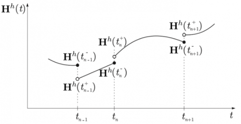
The method allows unknowns Hh(t) to be discontinuous across the interface of time intervals, and the approximations at time tn are written as:
$\mathbf{H}^{h}\left(t_{n}^{+}\right)=\lim _{\delta t \rightarrow 0} \mathbf{H}^{h}\left(t_{n}+\delta t\right) ; \delta t>0$ (39.1)
$\mathbf{H}^{h}\left(t_{n}^{-}\right)=\lim _{\delta t \rightarrow 0} \mathbf{H}^{h}\left(t_{n}-\delta t\right) ; \delta t>0$ (39.2)
An illustration of time discontinuous approximation is provided in Figure 3.
Figure 3. Time discontinuous approximation of solutions
In such discontinuous solutions, the jump operator across each time interface tn is defined as:
$\mathbf{H}^{h}\left(t_{n}\right)=\mathbf{H}^{h}\left(t_{n}^{+}\right)-\mathbf{H}^{h}\left(t_{n}^{-}\right)$ (40)
where, n=0, 1, 2, …, N-1. The principle of TDG-FEM [21] is to find $\mathbf{H}^{h}(t) \in \mathcal{V}^{h}$ such that for all $\mathbf{W}^{h}(t) \in \mathcal{V}^{h}$, such that:
$a\left(\mathbf{W}^{h}, \mathbf{H}^{h}\right)_{n}=l\left(\mathbf{W}_{n}^{h}\right)$ (41)
where,
$a\left(\mathbf{W}^{h}, \mathbf{H}^{h}\right)_{n}:=\left(\mathbf{W}^{h}, \mathbf{M} \dot{\mathbf{H}}^{h}\right)_{I_{n}}+\left(\mathbf{W}^{h}, \mathbf{D} \mathbf{H}^{h}\right)_{I_{n}}$$+\mathbf{W}^{h}\left(t_{n}^{+}\right) \cdot \mathbf{M H}^{h}\left(t_{n}^{+}\right)$ (42)
and
$l\left(\mathbf{W}_{n}^{h}\right):=\mathbf{W}^{h}\left(t_{n}^{+}\right) \cdot \mathbf{M} \mathbf{H}^{h}\left(t_{n}^{-}\right)$ (43)
in which Hh(t0)=H0. The L2-inner product for the time interval can be obtained as:
$\begin{aligned}(\mathbf{W}, \mathbf{H})_{I_{n}}=\int_{I_{n}} \mathbf{W H} d t &=\lim _{\delta t \rightarrow 0} \int_{t_{n}+\delta t}^{t_{n}+1-\delta t} \mathbf{W H} d t \\ \delta t &>0 \end{aligned}$ (44)
From Eq. (43), it can be seen that the solutions of $\mathbf{H}^{h}\left(t_{n}^{-}\right)$ from the end of the previous time step are to be used as initial conditions for the current time step. The approximations to H(t) are given as:
$\mathbf{H}^{h}(t)=\mathbf{H}_{n}^{-}+\left[\boldsymbol{\varphi}(t) \otimes \mathbf{I}_{n_{e q}}\right] \overline{\mathbf{H}}, t \in\left(t_{n}, t_{n+1}\right)$ (45)
where, $\mathbf{H}_{n}^{-}$ is a column vector of size neq, containing neq humidity values at the end of the previous time step, $\boldsymbol{\varphi}(t)=\left[\varphi_{0}(t), \varphi_{1}(t), \ldots, \varphi_{p}(t)\right]$- a row vector of size p+1, containing the time shape functions of each polynomial order, from 0 to p. $\overline{\mathbf{H}}=T\left[\overline{\mathbf{H}}_{0}, \overline{\mathbf{H}}_{1}, \ldots, \overline{\mathbf{H}}_{p}\right]$ - a column vector of size (p+1) neq, in which, each $\overline{\mathbf{H}}_{i}$ denotes the vector of undetermined coefficients corresponding to humidity, $\otimes$ represents the Kronecker (tensor) product, $\mathbf{I}_{n_{e q}}$ is the identity matrix of order neq.
As to achieve an optimally efficient iterative algorithm with high-order accuracy, the time shape functions are obtained thereby mapping of monomial basis {1, t, t2, …, tp}. The time interval, t is normalized to an interval $\hat{t} \in(0,1)$, using linear scaling, i.e. $t=t_{n}^{+}\left(\Delta t_{n}\right) \hat{t}$. For choices of time shape functions, we adopt those defined in Eq. (56) in a previous study [24], which reads:
$\varphi_{i}(\hat{t})=\sum_{k=0}^{i}(-1)^{k} k ! \hat{\gamma}^{k}\left(\begin{array}{l}i \\ k\end{array}\right)^{2} \hat{t}^{i-k}$ (46)
for i=0, 1, 2, …, p and $\left(\begin{array}{l}i \\ k\end{array}\right)$ denotes the binomial coefficient, $\hat{\gamma}=1 /(2 p+1)$.
By the substitution of the trial functions from Eq. (45) into Eq. (41), the coupled matrix equations for each time interval are obtained as:
$(A \otimes \mathbf{M}+B \otimes \mathbf{D}) \overline{\mathbf{H}}=-b \otimes \mathbf{M} \mathbf{H}_{n}^{-}$ (47)
where, A and B, of size (p+1)×(p+1), are defined as follows:
$A=\int_{0}^{1} T_{\boldsymbol{\varphi}}(\hat{t}) \dot{\boldsymbol{\varphi}}(\hat{t}) d \hat{t}+{ }^{T} \boldsymbol{\varphi}(0) \boldsymbol{\varphi}(0)$ (48)
$B={ }^{T} B=\Delta t_{n} \int_{0}^{1}{ }^{T} \boldsymbol{\varphi}(\hat{t}) \boldsymbol{\varphi}(\hat{t}) d \hat{t}$ (49)
and
$b=\Delta t_{n} \int_{0}^{1}{ }^{T} \boldsymbol{\varphi}(\hat{t}) d \hat{t}$ (50)
From above, the number of linear equations in Eq. (47) is (p+1) times larger than the system of the second order accurate SS/SS algorithm such as that of generalized trapezoidal method. Plus, direct solutions of the large system of coupled equations $\overline{\mathbf{H}}_{i}$ require high computational costs. In this work, we have adapted the numerical implementation proposed in [24] to solve first-order parabolic moisture diffusion equations. Taking Eq. (47) and multiplying both sides by ($A^{-} \otimes \mathbf{I}_{n_{e q}}$) yields:
$\left(I_{p+1} \otimes \mathbf{M}+W \otimes \mathbf{D}\right) \overline{\mathbf{H}}=-d \otimes \mathbf{M H}_{n}^{-}$ (51)
where, Ip+1 is the identity matrix of order p+1, W=A-1B and
$d=A^{-1} b=\Delta t_{n} \int_{0}^{1}={ }^{T}\left\{\hat{\gamma} \Delta t_{n}, \Delta t_{n}, 0,0, \ldots, 0\right\}$ (52)
Let D and E be the diagonal and off-diagonal parts of W; W=D+E, where $D=\gamma I_{p+1}=\widehat{\gamma} \Delta t I_{p+1}$, and
$E=\left[\begin{array}{llllll}0 & E_{01} & E_{02} & E_{03} & \ldots & E_{0 p} \\ E_{10} & 0 & E_{12} & E_{13} & \ldots & E_{1 p} \\ E_{20} & E_{21} & 0 & E_{23} & \ldots & E_{2 p} \\ E_{30} & E_{31} & E_{32} & 0 & \ldots & E_{3 p} \\ \vdots & \vdots & \vdots & \vdots & \ddots & \vdots \\ E_{p 0} & E_{p 1} & E_{p 2} & E_{p 3} & \ldots & 0\end{array}\right]$ (53)
To develop a predictor-corrector algorithm, the left-hand side of Eq. (51) is re-written as:
$\left(I_{p+1} \otimes[\mathbf{M}+\gamma \mathbf{D}]+E \otimes \mathbf{D}\right) \overline{\mathbf{H}}=-d \otimes \mathbf{M H}_{n}^{-}$ (54)
where, $\gamma=\widehat{\gamma} \Delta t$. To achieve for an efficient multi-pass algorithm, a Gauss-Seidel block matrix iterative scheme is employed. This is done by splitting matrix E into upper and lower triangular matrices, i.e., E=EU+EL. So, Eq. (54) can be re-written as:
|
Algorithm 1. Predictor/multi-corrector multi-pass algorithm at time t. |
|
Input: $\mathbf{M}^{*}, \mathbf{D}, \boldsymbol{\varphi}(\hat{t}), \gamma, E, p, l_{\max }$ Output: $\mathbf{H}_{t}^{h}$ $\mathbf{M}^{*} \leftarrow \mathbf{M}+\gamma \mathbf{D}$ Form effective mass matrix $\overline{\mathbf{H}}_{i}^{(0)} \leftarrow \mathbf{0}$ i=0, 1, 2, …, p for $l \leftarrow 1$ to lmax do for $i \leftarrow 1$ to p do $\widetilde{\mathbf{H}}_{i}^{(l)} \leftarrow \mathbf{H}_{n}^{-}+E_{i i-1}^{L} \overline{\mathbf{H}}_{i-1}^{(l)}+\sum_{j=i+1}^{p} E_{i j}^{U} \overline{\mathbf{H}}_{j}^{(l-1)}$ Predictor phase $\mathbf{M}^{*} \overline{\mathbf{H}}_{i}^{(l)} \leftarrow-\mathbf{D} \widetilde{\mathbf{H}}_{i}^{(l)}$ Corrector phase end for end for $\mathbf{H}_{n+1}^{-} \leftarrow \mathbf{H}_{n}^{-}+\sum_{i=0}^{p} \varphi_{i}(1) \overline{\mathbf{H}}_{i}$ Update solutions |
$\left(I_{p+1} \otimes[\mathbf{M}+\gamma \mathbf{D}]+E^{L} \otimes \mathbf{D}\right) \overline{\mathbf{H}}^{(l)}=-d \otimes \mathbf{M H}_{n}^{-}-E^{U} \otimes \mathbf{D} \overline{\mathbf{H}}^{(l-1)}$ (55)
where, l=1, 2, …, lmax, and $\overline{\mathbf{H}}^{(l)}$ denotes the solutions obtained from the lth iterate. With a given set of initial values, $\overline{\mathbf{H}}^{(0)}=0$ , Eq. (55) is repeated to determine $\overline{\mathbf{H}}^{\left(l_{\max }\right)}$. The solutions Hh(t) can then be calculated via Equation (45). The above iterative scheme is written in the form of the predictor/multi-corrector (v-form) multi-pass algorithm is summarised in Algorithm 1.
In order to investigate and ensure the stability and accuracy of the proposed algorithm, a homogeneous first-order problem with one degree of freedom is taken:
$\dot{H}(t)+\lambda H(t)=0 ; \quad t_{n}^{+} \leq t \leq t_{n+1}^{-}$ (56)
$H\left(t_{n}^{-}\right)=H_{n}^{-}$ (57)
For the current time step, the solutions at the end of the interval is written as:
$H^{h}\left(t_{n+}^{-}\right)=\mathcal{A}^{(l)} H^{h}\left(t_{n}^{-}\right)$ (58)
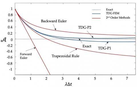
where, $\mathcal{A}^{(l)}$ is the amplification matrix at the lth iterate. The algorithm is considered unconditionally stable, i.e. A-stable, if $|\mathcal{A}|<1$ for all positive λΔtn. The graphs of amplification factor obtained by TDG-FEM and by second-order accurate methods as a function of normalized frequency, λΔtn are plotted in Figure 4. It shows that the solutions obtained by TDG-P2 are the most accurate, with reference to the exact solutions.
The accuracy of the algorithm is measured by replacing Hh in Eq. (58) by exact values H. Then, the local truncation error of solution in each iteration pass l at the end of time step tn is given as:
$\varepsilon^{(l)}=H\left(t_{n+1}^{-}\right)-{ }_{\mathcal{A}}^{(l)} H\left(t_{n}^{-}\right)$ (59)
and by using the Taylor’s series at about Δt=0 to obtain the expansion of Eq. (59), the local order accuracy is defined as:
$\tau^{(l)}\left(t_{n}\right)=C_{k} \Delta t^{k}+C_{k+1} \Delta t^{k+1}+\ldots$ (60)
where, C are time-independent coefficients. The consistency of algorithm is measured as the order of k where k>0 and $|\tau(t)| \leq C_{k} \Delta t^{k}$ for $t \in\left[0, t_{f}\right]$. The orders of accuracy achieved by the proposed iterative algorithms of linear, when p=1, and quadratic, when p=2, are illustrated in Table 1.
Table 1. Accuracy and stability of iterative algorithms
|
Algorithm |
lmax |
Error Rate |
|Ck| |
Stability |
|
TDG-P1 |
1 |
Δt |
0.05556 |
A-stable |
|
2 |
Δt3 |
0.01698 |
A-stable |
|
|
3 |
Δt3 |
0.01389 |
A-stable |
|
|
Direct Solution |
Δt3 |
0.01389 |
A-stable |
|
|
TDG-P2 |
1 |
Δt2 |
0.02133 |
A-stable |
|
2 |
Δt4 |
0.00064 |
A-stable |
|
|
3 |
Δt5 |
0.00014 |
A-stable |
|
|
Direct Solution |
Δt5 |
0.00014 |
A-stable |
The iterative algorithms of TDG-P1 and TDG-P2 methods require three iteration passes (lmax=3) to achieve the same orders of accuracy and coefficients as that calculated by direct solving. Therefore, a high order of accuracy obtained by only a few iterations passes means that the algorithm is efficient and stable.
Figure 4. Amplification factors of different methods
3.3 Adaptive time-stepping method
Usually, moisture diffusion occurs in a very extended period of time in normal environmental conditions. This means that the smaller the time step, the more expensive the calculations. To minimise the simulation time with reliable accuracy, we employ the embedded pair approach. This method has been successfully implemented in the Runge-Kutta methods [30-32], where the resulting parameters determined by the higher-order (q) accurate algorithm are used in the algorithm with a lower order (r) of accuracy.
From Table 1, since our TDG-P2 iterative method with three passes, i.e., TDG-P2(3) yields the optimal accuracy, the embedded solutions are, hence, of a lower-order accuracy with two passes, i.e., TDG-P2(2) such that r=q-1. The difference:
$\mathbf{e}=\mathbf{H}_{n+1}^{-}-\widehat{\mathbf{H}}_{n+1}^{-}$ (61)
is used as a local error estimate, where $\mathbf{H}_{n+1}^{-}$ and $\widehat{\mathbf{H}}_{n+1}^{-}$ are the solutions by TDG-P2(3) and TDG-P2(2) respectively. Using the standard rule to predict the new step size [33-35] leads to:
$\Delta t_{n+1}=\alpha \Delta t_{n}\left(\frac{\eta_{\text {tol }}}{\eta}\right)^{1 / p}$ (62)
where, α is a safety factor, and p=2 for TDG-P2. ηtol is the specified tolerance being equal to 0.1% in this work, and η is the relative local error estimate:
$\eta=\frac{\|\mathbf{e}\|_{E}}{\|\mathbf{U}\|_{E}} \times 100 \%$ (63)
Using the error measured in total energy norm, the estimated local error becomes:
$\|\mathbf{e}\|_{E}=\left({ }^{T} \mathbf{e} \mathbf{D} \mathbf{e}\right)^{1 / 2}$ (64)
and, thus, $\|\mathbf{U}\|_{E}$ is the maximum total energy norm recorded during the simulation:
$\|\mathbf{U}\|_{E}=\max _{i=0,1, \ldots, n+1}\left({ }^{T} \mathbf{H}_{i}^{-} \mathbf{D} \mathbf{H}_{i}^{-}\right)^{1 / 2}$ (65)
To make the time stepping method efficient and reliable, the new step size Δtn+1 from Eq. (62) is accepted only when η<ηtol. Also, to avoid drastic changes in step size, the limit of time step change is imposed, i.e., Δtn+1≤βΔtn, in which β is the control factor, which is taken as 4 in this work. In the case where the error does not satisfy the criterion, i.e. η>ηtol, the updated solutions from the current step are rejected, and the determination of $\mathbf{H}_{n+1}^{-}$ is attempted with the new smaller step size Δtn+1.
3.4 Material parameters and conditions
The orthotropic elastic constants of wood fibers are determined, using the model proposed by Charupeng and Kunthong [36]. The model requires bulk density and lignocellulosic composition of wood fibers, and completely estimates all the essential elastic constants of wood fibers. Then, the formulation of FE equations in 3-D space for the initial configuration (t=0) are constructed, using representative volume element method (RVE), as shown in Figure 5(a). This method has been proven to be reliable with modeling the mechanical properties of wood fiber composites [37-40]. With a given value of ϕ and densities of matrix and fibers, the physical parameters a, b, c, T and L can be determined. However, the full RVE model is rather expensive to simulate and unnecessary. We, instead, use a reduced model which is split about the three planes of symmetry in Cartesian system, as depicted in Figure 5(b). This reduces the total number of elements in calculations by a factor of 8.
The geometrical parameters shown in Figure 5(a) can be determined as follows. The volume fraction of fiber is determined from basic materials properties as:
$f=\frac{\frac{w_{f}}{\rho_{f}}}{\frac{w_{f}}{\rho_{f}}+\frac{1-w_{f}}{\rho_{m}}}$ (66)
where, wf and ρf are the weight fraction and bulk density of wood fibers, ρm is the density of matrix material.
The volume fraction is then used to approximate the initial geometrical parameters a and b of the model - for a constant thickness of fiber wall, a=b=t. The parameter c is determined by averaging the element sizes along the x and y direction. Given the volume of model V, fiber width ϕ and width-to-thickness ration; k=ϕ/T, the average element size along the fiber direction c=L/Nz; Nz is the number of elements along the fiber direction, and $L=\frac{V}{(\phi+2 a)(\phi / k+2 b)}\quad.$ Finally, the corrected value of t is determined via:
$f=\frac{\phi^{2}(L-2 c)}{k(\phi+2 t)(\phi / k+2 t)}$ (67)
where, according to literature [41], k=2.
In each complete iteration, the development of moisture, i.e., ΔH calculated by the aforementioned algorithm in Algorithm 1, gives rise to non-zero components in matrix F of Eq. (36). With the pre-defined global stiffness matrix K, the global displacements U are determined, and hence used to update the physical coordinates of the domain. This process is repeated until the simulation time is reached. The final geometry is post-processed to obtain meaningful results.
All the linear systems of equations are solved by preconditioned conjugate gradient (PCG) method [42]. This method offers a relatively short period of time to converge and good reliability in solving symmetric positive definite matrices. The convergence of PCG calculation is ensured by setting the tolerance to 1×10⁻⁷ and the maximum iteration number at 10,000. which are then used to update the physical coordinates for the next time step.
In order to illustrate a numerical example as well as validate the algorithm, the experimental results in Ref. [5] are taken for comparison. There are two matrix polymers: polylactic acid (PLA) and polypropylene (PP). The fibers are bleached birch kraft fibers. The essential material parameters are summarised in Table 2. The properties of polymers are assumed to be isotropic. The diffusion coefficients and elastic constants are assumed to be independent upon moisture absorption.
Table 2. Parameter inputs. Referenced studies from which values are taken are included. %C, %H and %L denote the weight fractions of cellulose, hemicellulose and lignin respectively
|
Constituent |
Parameter |
Value |
Ref. |
|
Birch |
ρ(kgm-3) |
690 |
[43] |
|
%C |
71.7 |
[43] |
|
|
%H |
26.1 |
[43] |
|
|
%L |
2.0 |
[43] |
|
|
ϕ(μm) |
21.3 |
[44] |
|
|
Dh,x(10-12m2s-1) |
2.26 |
[45] |
|
|
Dh,y(10-12m2s-1) |
2.26 |
[45] |
|
|
Dh,z(10-12m2s-1) |
5.65 |
[45] |
|
|
PLA |
ρ(kgm-3) |
1230 |
[46] |
|
E(GPa) |
1.93 |
[46] |
|
|
ν |
0.35 |
[47] |
|
|
D(10-13m2s-1) |
1.77 |
[48] |
|
|
∂W/∂H |
1×10⁻² |
[49] |
|
|
PP |
ρ(kgm-3) |
925 |
[50] |
|
E(GPa) |
1.6 |
[51] |
|
|
ν |
0.45 |
[52] |
|
|
D(10-13m2s-1) |
1.90 |
[53] |
|
|
∂W/∂H |
8×10⁻⁴ |
[54] |
The hygroexpansion coefficient is generally very small in polymeric materials [3, 55] compared to that of wood, and hence assumed to be zero. As the moisture capacity of fiber usually varies with relative humidity, we employ the Guggenheim-Andersen-de Boer (GAB) three-parameter sorption Eq. [56], in which the equilibrium moisture content in cellulose fibers can be determined via:
$W=\frac{V_{m} \times c \times k \times H / 100}{(1-k \times H / 100)(1+(c-1) k \times H / 100)}$ (68)
where, H is the relative humidity, and for adsorption parameters of birch wood, Vm=0.058, c=8.9, k=0.78 [57]. So, ∂W/∂H, can be determined by differentiating Eq. (68).
Also, by using the FE algorithm [36] with inputs from Table 2 -ρ, %C, %H and %L, the elastic constants of wood fibers are estimated and summarised in Table 3. The above properties of the homogenised fiber model are used to simulate the birch pulp in the experiments [5].
Table 3. Elastic constants of homogenised birch fibers
|
$E_{x}$ (GPa) |
$E_{y}$ (GPa) |
$E_{z}$ (GPa) |
$G_{y z}$ (GPa) |
$G_{zx}$ (GPa) |
$G_{xy}$ (GPa) |
$\nu_{z y}$ |
$\nu_{z x}$ |
$\nu_{x y}$ |
|
2.62 |
2.62 |
42.8 |
4.23 |
4.23 |
1.19 |
0.447 |
0.447 |
0.104 |
Figure 5. RVE model of WPC; fiber(brown), matrix(yellow). (a) full model with annotated multi-view projection. (b) actual physical domain used for simulation. ϕ, T and L are the width, thickness and length of the homogenised fiber respectively
With reference to Figure 5(b), the boundary conditions imposed at all time steps are:
$\mathbf{H}(\infty, y, z)=\mathbf{H}(x, \infty, z)=\mathbf{H}(x, y, \infty)=R H$ (69)
$\mathbf{u}(0, y, z)=\mathbf{v}(x, 0, z)=\mathbf{w}(x, y, 0)=0$ (70)
where, RH is the relative humidity, u, v and w are nodal displacements along the x, y and z directions, and ∞ indicates the boundary on a specific dimension. In other words, Eq. (69) are posed on to the nodes with coordinates $\left(\frac{\phi}{2}+a, y, z\right),\left(x, \frac{T}{2}+b, z\right)$, and $\left(x, y, \frac{L}{2}+c\right)$ where ϕ, T, L, a, b, c are parameters according to Figure 5(a). And from Eq. (70), u=0 are posed on to the nodes with coordinates (0, y, z), v=0 are posed on to the nodes with coordinates (x, 0, z), and w=0 are posed on to the nodes with coordinates (x, y, 0).
The initial conditions from Eq. (20) are used on all nodes except that with the imposed essential conditions above.
As for the FE discretisation, the dimensions of the RVE model are specified such that the total volume of the model equals the total volume of the specimens in the experiments. The uniformity of mesh is ensured by making all element as close to a square as possible. Using the concepts of RVE, the average out-of-plane hygroexpansion, is plotted against time for convergence tests as shown in Figure 6.
Figure 6. Effects of mesh geometry on the solutions obtained for 30% birch and 70% PP by weight, at RH=0.97. 3×2×10 indicates that the FE model has three elements, two elements and 10 elements along the x, y and z respectively
The choices of cross-sectional dimensions xy-planes of elements are rather limited as to conserve the volume fraction of fiber and the fiber width-to-thickness ratio W/T. Refining the mesh from 2×2×10 to 3×2×10 and increasing the number of elements along the fiber direction yield converged solutions to less than 1% as the dimensions of each element become more uniform. However, the 4×3×13 mesh has the greatest number of elements but yields a rather different trend of solutions. This is because, in order to conserve the volume fraction of fibers, such mesh leads to uneven dimensions of elements on the cross-sections, and hence poor aspect ratios. Therefore, the minimum refinement of mesh is 3 by 2 by 12 elements.
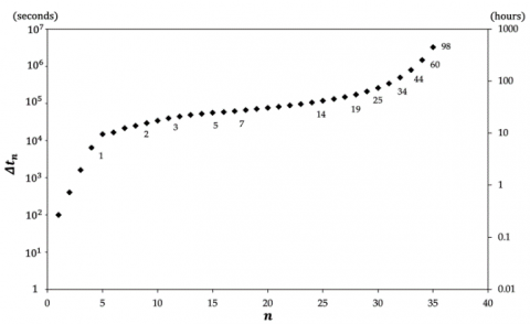
The preferred mesh refinement is taken for the evaluation of the efficiency of time-stepping algorithm. The initial time step is set to 100 seconds with β=4 to avoid large increases of step size, α=0.9 and ηtol=0.1%. The size of time step, Δtn, are plotted against iteration number, n, as shown in Figure 7.
Figure 7. Time step progression vs step number. Labels of approximate day number in the simulated period are included for certain iterations. Runtime is approximately 6.5 hours
The results show that the step size rises rather rapidly for the first few steps to a certain range - around 104 seconds or three hours. It then increases from hours to days and weeks, as implied by the labelled day numbers. Such increasing intervals are also used commonly by numerous similar experimental studies [5-7]. This suggests that the algorithm quickly determines the appropriate step size from the solutions and progresses according to the hygro-mechanical behaviours. The fact that our algorithm requires 6.5 hours of runtime to simulate the actual period of 90 days indicates good robustness and its potential for industrial applications - predictions of dimensional stability and hence durability of materials are essential but expensive for laboratory experiments.
Figure 8 shows the predicted time-dependent out-of-plane hygroexpansion as a function of time, for a series of different fiber volume fractions and material constituents. All FE calculations are performed with RH=0.97, Δt1=100s, α=0.9, ηtol=0.1% and β=4. The results are compared to corresponding experimental results.
Figure 8. Time-dependent out-of-plane hygroexpansion predicted by our FEA model (solid lines) compared to the experiments [5] (dotted lines)
There is good agreement between our FEA calculations and the results of the experiments [5]. The model accurately predicts accurately the hygroexpansion towards equilibrium moisture content with slight differences of up to 10% in the first 10-20 days. Within the aforementioned period, the reliability of the prediction is slightly lower, which is due to the fact that the magnitude of the diffusion coefficient in polymers can vary from 10-15 to 10-11 m2/s [58, 59]. Moreover, water absorption, although very small, can lead to rearrangement of the chemical chains and thus to a change in diffusivity [2].
While the numerical model assumes perfect interfaces between the fibers and the matrix, this is usually not the case in practice. The interfacial compatibility of wood fibers is poor in a PP matrix but strong in a PLA matrix, as evidenced by SEM micrographs according to the literature [5, 60]. Thus, as hygroexpansion progresses, microcracks and interfacial debonding develop, providing more channels for a greater extent of moisture diffusion. This has also been shown by Suri and Perreux [61] that damage and cracks lead to increased water diffusion rate in fiber composites. As a result, FEA calculations give higher values compared to the experiments in the case of 30 wt% fibers and 70 wt% PP after 20 days.
It should also be noted that the simulation environments are assumed such that all the sides (boundary surfaces) of composite specimens are exposed to uniform relative humidity and that the specimen are kept at constant and standard temperature and pressure during the diffusion process. In terms of actual experimentation, the consistency with of such conditions is ensured by complying to the relevant standard ASTM D 570-81 [5].
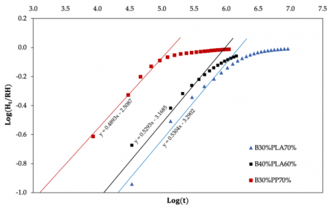
To further evaluate the reliability and accuracy of the modeling methods, the kinetics of diffusion is analysed. The analytical equation describing the diffusion mechanism and kinetics can be given as follows:
$\log \left(\frac{M_{t}}{M_{\infty}}\right)=\log (k)+n \log (t)$ (71)
where, Mt and M∞ denote moisture content at time t and that at the equilibrium respectively, k and n are constants [62]. For relative moistures of lower than 0.5 (Mt/M∞≤0.5), the n value indicates the type of diffusion mechanism; n=0.5 for general Fickian diffusion processes [63]. Here, the value of Mt/M∞ is assumed to be equal to Ht/RH. The value of Ht is given by the average value of the nodal solutions from Eq. (37) at time t. Since the equilibrium value cannot exceed the relative humidity RH (see Eq. (19)), this value is set as the equilibrium value.
Figure 9. Log of relative moisture against log time in seconds including trend lines
Figure 9 shows log(Ht/RH) as a function of log(t) for the three composites. For all composites, the slopes of the trend line, i.e. n, are approximately equal to 0.5 - with a deviation of at most 6%. This is in agreement with the experimental study [6], according to which numerous natural fibers/ PP composites have n value of about 0.5, thus obeying the kinetics theory of a Fickian diffusion process. There is a slight difference between the log(k) values from the trend line equations of birch fiber/PLA composites because the RVE models are dimensioned differently due to the difference in fiber weight fractions. Moreover, the n value for birch fiber/PP composites is quite different due to the low interfacial compatibility mentioned earlier. The above analysis confirms that our model can effectively capture the physics of the hygro-mechanical behaviours of WPC as well as the kinetics according to Fick’s theory.
We have successfully developed a validated finite element model based on semi-discretization of space and time to study the three-dimensional hygro-mechanical behaviours of wood fiber-polymer composites. The solutions are continuous in space but can be discontinuous in time, using TDG-FEM for the latter to achieve optimal accuracy.
A predictor/multi-corrector using a Gauss-Seidel block matrix iterative scheme algorithm for solving the first-order parabolic problem in temporal domain has also been presented. It requires only up to three iterative passes to achieve the same accuracy as the direct solution. Moreover, the adaptive time-stepping method using embedded solution approach with the maximum energy norm criterion has been shown to effectively determine the appropriate size of time step and to progress efficiently throughout the simulation period. A runtime of a few hours compared to about three months of actual laboratory experiments confirms the efficiency and robustness in predicting the complex time-dependent hygro-mechanical behaviours.
As for the validation of the model, the FEA results are compared with the corresponding cases in previous experimental studies and show good agreement. The reliability of the prediction can increase with the interfacial compatibility between fiber and matrix. Diffusion at early stages may be more difficult to predict due to the variability of material parameters in polymeric materials. Data analysis of the time-dependent moisture content confirms that Fick’s theory is very good at predicting the behaviours, with the characteristic n value in agreement with experiments.
[1] Bledzki, A.K., Sperber, V.E., Faruk, O. (2002). Natural and wood fibre reinforcement in polymers. iSmithers Rapra Publishing.
[2] Weisenberger, L.A., Koenig, J.L. (1989). NMR imaging of solvent diffusion in polymers. Applied Spectroscopy, 43(7): 1117-1126.
[3] Yew, G.H., Yusof, A.M., Ishak, Z.M., Ishiaku, U.S. (2005). Water absorption and enzymatic degradation of poly (lactic acid)/rice starch composites. Polymer Degradation and Stability, 90(3): 488-500. https://doi.org/10.1016/j.polymdegradstab.2005.04.006
[4] Klyosov, A.A. (2007). Wood-Plastic Composites. John Wiley & Sons, 1-698. https://doi.org/10.1002/9780470165935
[5] Almgren, K.M., Gamstedt, E.K., Berthold, F., Lindström, M. (2009). Moisture uptake and hygroexpansion of wood fiber composite materials with polylactide and polypropylene matrix materials. Polymer Composites, 30(12): 1809-1816. https://doi.org/10.1002/pc.20753
[6] Espert, A., Vilaplana, F., Karlsson, S. (2004). Comparison of water absorption in natural cellulosic fibres from wood and one-year crops in polypropylene composites and its influence on their mechanical properties. Composites Part A: Applied Science and Manufacturing, 35(11): 1267-1276. https://doi.org/10.1016/j.compositesa.2004.04.004
[7] Leu, Y.Y., Chow, W.S. (2011). Kinetics of water absorption and thermal properties of poly (lactic acid)/organomontmorillonite/poly (ethylene glycol) nanocomposites. Journal of Vinyl and Additive Technology, 17(1): 40-47. https://doi.org/10.1002/vnl.20259
[8] Duanmu, J., Gamstedt, E.K., Rosling, A. (2007). Hygromechanical properties of composites of crosslinked allylglycidyl-ether modified starch reinforced by wood fibres. Composites Science and Technology, 67(15-16): 3090-3097. https://doi.org/10.1016/j.compscitech.2007.04.027
[9] Šejnoha, M., Sýkora, J., Vorel, J., Kucíková, L., Antoš, J., Pokorný, J., Pavlík, Z. (2019). Moisture induced strains in spruce from homogenization and transient moisture transport analysis. Computers & Structures, 220: 114-130. https://doi.org/10.1016/j.compstruc.2019.04.008
[10] Autengruber, M., Lukacevic, M., Füssl, J. (2020). Finite-element-based moisture transport model for wood including free water above the fiber saturation point. International Journal of Heat and Mass Transfer, 161: 120228. https://doi.org/10.1016/j.ijheatmasstransfer.2020.120228
[11] Wang, N., Liu, W., Lai, J. (2014). An attempt to model the influence of gradual transition between cell wall layers on cell wall hygroelastic properties. Journal of Materials Science, 49(5): 1984-1993. https://doi.org/10.1007/s10853-013-7885-5
[12] Joffre, T., Isaksson, P., Dumont, P.J., Roscoat, S., Sticko, S., Orgéas, L., Gamstedt, E.K. (2016). A method to measure moisture induced swelling properties of a single wood cell. Experimental Mechanics, 56(5): 723-733. https://doi.org/10.1007/s11340-015-0119-9
[13] Obeid, H., Clément, A., Fréour, S., Jacquemin, F., Casari, P. (2018). On the identification of the coefficient of moisture expansion of polyamide-6: Accounting differential swelling strains and plasticization. Mechanics of Materials, 118: 1-10. https://doi.org/10.1016/j.mechmat.2017.12.002
[14] Sar, B.E., Fréour, S., Célino, A., Jacquemin, F. (2015). Accounting for differential swelling in the multi-physics modeling of the diffusive behavior of a tubular polymer structure. Journal of Composite Materials, 49(19): 2375-2387. https://doi.org/10.1177%2F0021998314546704
[15] Sar, B.E., Fréour, S., Davies, P., Jacquemin, F. (2014). Accounting for differential swelling in the multi-physics modelling of the diffusive behaviour of polymers. ZAMM-Journal of Applied Mathematics and Mechanics/Zeitschrift für Angewandte Mathematik und Mechanik, 94(6): 452-460. https://doi.org/10.1002/zamm.201200272
[16] Mbacké, M.A., Khazaie, S., Fréour, S., Jacquemin, F. (2020). Numerical modeling of the hygro-mechanical behavior of the 3D composite materials. Journal of Composite Materials, 54(28): 4457-4471. https://doi.org/10.1177%2F0021998320932270
[17] Youssef, G., Fréour, S., Jacquemin, F. (2009). Stress-dependent moisture diffusion in composite materials. Journal of Composite Materials, 43(15): 1621-1637. https://doi.org/10.1177%2F0021998309339222
[18] Stahl, D.C., Cramer, S.M. (1998). A three-dimensional network model for a low density fibrous composite. J. Eng. Mater. Technol., 120(2): 126-130. https://doi.org/10.1115/1.2807000
[19] Termonia, Y. (1994). Structure-property relationships in short-fiber-reinforced composites. Journal of Polymer Science Part B: Polymer Physics, 32(6): 969-979. https://doi.org/10.1002/polb.1994.090320601
[20] Hughes, T.J. (2012). The Finite Element Method: Linear Static and Dynamic Finite Element Analysis. Dover Publication, Inc.
[21] Hughes, T.J., Hulbert, G.M. (1988). Space-time finite element methods for elastodynamics: Formulations and error estimates. Computer Methods in Applied Mechanics and Engineering, 66(3): 339-363. https://doi.org/10.1016/0045-7825(88)90006-0
[22] Chien, C.C., Wu, T.Y. (2000). An improved predictor/multi-corrector algorithm for a time-discontinuous Galerkin finite element method in structural dynamics. Computational Mechanics, 25(5): 430-437. https://doi.org/10.1007/s004660050490
[23] Zhang, R., Wen, L., Xiao, J., Qian, D. (2019). An efficient solution algorithm for space–time finite element method. Computational Mechanics, 63(3): 455-470. https://doi.org/10.1007/s00466-018-1603-8
[24] Kunthong, P., Thompson, L.L. (2005). An efficient solver for the high-order accurate time-discontinuous Galerkin (TDG) method for second-order hyperbolic systems. Finite Elements in Analysis and Design, 41(7-8): 729-762. https://doi.org/10.1016/j.finel.2004.09.003
[25] Sharma, V., Fujisawa, K., Murakami, A. (2021). Space-time finite element method for transient and unconfined seepage flow analysis. Finite Elements in Analysis and Design, 197: 103632. https://doi.org/10.1016/j.finel.2021.103632
[26] Luo, H., Absillis, G., Nourgaliev, R. (2021). A moving discontinuous Galerkin finite element method with interface condition enforcement for compressible flows. Journal of Computational Physics, 445: 110618. https://doi.org/10.1016/j.jcp.2021.110618
[27] Baccouch, M., Temimi, H. (2021). A high-order space–time ultra-weak discontinuous Galerkin method for the second-order wave equation in one space dimension. Journal of Computational and Applied Mathematics, 389: 113331. https://doi.org/10.1016/j.cam.2020.113331
[28] Dong, Z., Li, H. (2021). A space-time finite element method based on local projection stabilization in space and discontinuous Galerkin method in time for convection-diffusion-reaction equations. Applied Mathematics and Computation, 397: 125937. https://doi.org/10.1016/j.amc.2020.125937
[29] MATLAB, V9.10.0.1739362 (R2021a). 2021, Massachusetts: The MathWorks, Inc.
[30] Dormand, J.R., El-Mikkawy, M.E.A., Prince, P.J. (1987). Families of Runge-Kutta-Nystrom formulae. IMA Journal of Numerical Analysis, 7(2): 235-250. https://doi.org/10.1093/imanum/7.2.235
[31] Higham, D.J. (1997). Regular Runge-Kutta pairs. Applied Numerical Mathematics, 25(2-3): 229-241. https://doi.org/10.1016/S0168-9274(97)00062-7
[32] de Swart, J.J., Söderlind, G. (1997). On the construction of error estimators for implicit Runge-Kutta methods. Journal of Computational and Applied Mathematics, 86(2): 347-358. https://doi.org/10.1016/S0377-0427(97)00166-0
[33] Gear, C.W. (1966). The numerical integration of ordinary differential equations of various orders (No. ANL-7126). Argonne National Lab., Ill. https://doi.org/10.1090/S0025-5718-1967-0225494-5
[34] Tsitouras, C., Papakostas, S.N. (1999). Cheap error estimation for Runge--Kutta methods. SIAM Journal on Scientific Computing, 20(6): 2067-2088. https://doi.org/10.1137/S1064827596302230
[35] Hull, T.E., Enright, W.H., Fellen, B.M., Sedgwick, A.E. (1972). Comparing numerical methods for ordinary differential equations. SIAM Journal on Numerical Analysis, 9(4): 603-637. https://doi.org/10.1137/0709052
[36] Charupeng, N., Kunthong, P. (2021). A novel finite element algorithm for predicting the elastic properties of wood fibers. International Journal of Computational Materials Science and Engineering, 2150027. https://doi.org/10.1142/S2047684121500275
[37] Shokrieh, M.M., Moshrefzadeh-Sani, H. (2016). An optimized representative volume element to predict the stiffness of aligned short fiber composites. Journal of Composite Materials, 50(23): 3301-3310. https://doi.org/10.1177%2F0021998315618456
[38] Ogierman, W., Kokot, G. (2018). Generation of the representative volume elements of composite materials with misaligned inclusions. Composite Structures, 201: 636-646. https://doi.org/10.1016/j.compstruct.2018.06.086
[39] Naderi, M., Apetre, N., Iyyer, N. (2017). Effect of interface properties on transverse tensile response of fiber-reinforced composites: three-dimensional micromechanical modeling. Journal of Composite Materials, 51(21): 2963-2977. https://doi.org/10.1177%2F0021998316681189
[40] Schneider, M. (2017). The sequential addition and migration method to generate representative volume elements for the homogenization of short fiber reinforced plastics. Computational Mechanics, 59(2): 247-263. https://doi.org/10.1007/s00466-016-1350-7
[41] Mansfield, S.D., Kibblewhite, R.P., Riddell, M.J. (2004). Characterization of the reinforcement potential of different softwood kraft fibers in softwood/hardwood pulp mixtures. Wood and Fiber Science, 36(3): 344-358.
[42] Barrett, R., Berry, M., Chan, T.F., Demmel, J., Donato, J., Dongarra, J., Eijkhout, V., Pozo, R., Romine, C., van der Vorst H. (1996). Templates for the solution of linear systems: Building blocks for iterative methods. Math. Comput., 64(211): 1349-1352. https://doi.org/10.2307/2153507
[43] Asikainen, S.A., Fuhrmann, A., Ranua, M., Robertsén, L. (2010). Effect of birch kraft pulp primary fines on bleaching and sheet properties. BioResources, 5(4): 2173-2183.
[44] Danielewicz, D., Surma-Ślusarska, B. (2017). Properties and fibre characterisation of bleached hemp, birch and pine pulps: A comparison. Cellulose, 24(11): 5173-5186. https://doi.org/10.1007/s10570-017-1476-6
[45] Šejnoha, M., KUCíKOVÁ, L., Vorel, J., Sýkora, J., De Wilde, W.P. (2019). Effective material properties of wood based on homogenization. International Journal of Computational Methods and Experimental Measurements, 7(2): 167-180. http://doi.org/10.2495/CMEM-V7-N2-167-180
[46] Van de Velde, K., Kiekens, P. (2002). Biopolymers: overview of several properties and consequences on their applications. Polymer Testing, 21(4): 433-442. https://doi.org/10.1016/S0142-9418(01)00107-6
[47] Fung, Y.C. (1965). Foundations of Solid Mechanics. New Jersey: Prentice-Hall, Inc.
[48] Yang, C., Xing, X., Li, Z., Zhang, S. (2020). A comprehensive review on water diffusion in polymers focusing on the polymer–metal interface combination. Polymers, 12(1): 138. https://doi.org/10.3390/polym12010138
[49] Cairncross, R.A., Becker, J.G., Ramaswamy, S., O’Connor, R. (2006). Moisture sorption, transport, and hydrolytic degradation in polylactide. In Twenty-Seventh Symposium on Biotechnology for Fuels and Chemicals, pp. 774-785. https://doi.org/10.1385/ABAB:131:1:774
[50] Maddah, H. A. (2016). Polypropylene as a promising plastic: A review. American Journal of Polymer Science, 6(1): 1-11. https://doi.org/10.5923/j.ajps.20160601.01
[51] Oksman, K., Skrifvars, M., Selin, J.F. (2003). Natural fibres as reinforcement in polylactic acid (PLA) composites. Composites science and technology, 63(9): 1317-1324. https://doi.org/10.1016/S0266-3538(03)00103-9
[52] Kumar, M., Gaur, K.K., Shakher, C. (2015). Measurement of material constants (Young's modulus and Poisson's ratio) of polypropylene using digital speckle pattern interferometry (DSPI). Journal of the Japanese Society for Experimental Mechanics, 15: s87-s91. https://doi.org/10.11395/jjsem.15.s87
[53] Yi, X., Pellegrino, J. (2002). Diffusion measurements with Fourier transform infrared attenuated total reflectance spectroscopy: Water diffusion in polypropylene. Journal of Polymer Science Part B: Polymer Physics, 40(10): 980-991. https://doi.org/10.1002/polb.10161
[54] Suherman, S., Peglow, M., Tsotsas, E. (2010). Measurement and modelling of sorption equilibrium curve of water on PA6, PP, HDPE and PVC by using Flory-Huggins model. Reaktor, 13(2): 89-94. https://doi.org/10.14710/reaktor.13.2.89-94
[55] Weitsman, Y.J. (2011). Fluid Effects in Polymers and Polymeric Composites. Springer Science & Business Media. http://doi.org/10.1007/978-1-4614-1059-1
[56] Timmermann, E.O. (2003). Multilayer sorption parameters: BET or GAB values? Colloids and Surfaces A: Physicochemical and Engineering Aspects, 220(1-3): 235-260. https://doi.org/10.1016/S0927-7757(03)00059-1
[57] Bratasz, Ł., Kozłowska, A., Kozłowski, R. (2012). Analysis of water adsorption by wood using the Guggenheim-Anderson-de Boer equation. European Journal of Wood and Wood Products, 70(4): 445-451. https://doi.org/10.1007/s00107-011-0571-x
[58] Duval, S., Camberlin, Y., Glotin, M., Keddam, M., Ropital, F., Takenouti, H. (2000). Characterisation of organic coatings in sour media and influence of polymer structure on corrosion performance. Progress in Organic Coatings, 39(1): 15-22. https://doi.org/10.1016/S0300-9440(00)00094-1
[59] De Rosa, L., Monetta, T., Bellucci, F. (1998). Moisture uptake in organic coatings monitored with EIS. Materials Science Forum, 289: 315-326. https://doi.org/10.4028/www.scientific.net/MSF.289-292.315
[60] Huda, M.S., Drzal, L.T., Misra, M., Mohanty, A.K. (2006). Wood-fiber-reinforced poly (lactic acid) composites: Evaluation of the physicomechanical and morphological properties. Journal of Applied Polymer Science, 102(5): 4856-4869. https://doi.org/10.1002/app.24829
[61] Suri, C., Perreux, D. (1995). The effects of mechanical damage in a glass fibre/epoxy composite on the absorption rate. Composites Engineering, 5(4): 415-424. https://doi.org/10.1016/0961-9526(94)00014-Z
[62] Comyn, J. (Ed.). (1985). Polymer Permeability. Springer Science & Business Media. http://doi.org/10.1007/978-94-009-4858-7
[63] Crank, J. (1956). The Mathematics of Diffusion. Oxford, UK: Cambridge University Press.