Ram Kishun Lodhi | Bharat Raj Jaiswal | Durgesh Nandan* | Katta Ramesh
© 2021 IIETA. This article is published by IIETA and is licensed under the CC BY 4.0 license (http://creativecommons.org/licenses/by/4.0/).
OPEN ACCESS
In this study, we have developed a fourth order compact finite difference method for finding the numerical solution of two-parameter singularly perturbed convection-diffusion boundary value problems. We have used fourth order compact finite difference method on uniform mesh which provides a tridiagonal linear system of equations. The convergence analysis of the proposed method is established through a matrix analysis approach and it is proved that present method gives fourth order convergence results. Present method is implemented on two numerical examples for checking the efficiency and precision of the method. Numerical outcomes are exhibited which supports the theoretical outcomes. Numerical outcomes are compared with other existing methods and found that present method gives more accurate approximate solution as compare to the other existing methods.
compact finite difference method, convection-diffusion, singular perturbation, two-parameter, uniform mesh
We consider the following two-parameter singularly perturbed convection--diffusion boundary value problem:
$-\varepsilon {u}''\left( x \right)+\mu p\left( x \right){u}'\left( x \right)+q\left( x \right)u\left( x \right)=f\left( x \right),\,x\in \left( 0,\,\,1 \right)$ (1)
$u\left( 0 \right)=\alpha ,\,u\left( 1 \right)=\beta .$ (2)
with two small positive parameters, $0<\varepsilon \ll 1$ and $0<\mu \ll 1$. The function $p(x), q(x)$ are sufficiently smooth real valued function and satisfied $p(x) \geq p^{*}>0, q(x) \geq q^{*}>0$ for $x \in(0,1)$. Under these assumptions problem (1) is characterized into two cases:
1) When we put $\mu=0$, in Eq. (1), then the Eq. (1) is known as reaction-diffusion singular perturbation problem.
2) When we put $\mu=1$, in Eq. (1), then the Eq. (1) is known as convection-diffusion singular perturbation problem.
These kinds of problems arise in numerous field like applied mathematics, chemical reactor theory and control theory [1-6]. O’Malley [7] has discussed the nature of two-parameter problems by asymptotic expansion where the ratio of $\mu$ and $\varepsilon$ have significant role in solution. The two-parameter singular perturbation boundary value problems have two cases $\frac{\mu^{2}}{\varepsilon \rightarrow 0}$ as $\varepsilon \rightarrow 0$ and $\frac{\varepsilon}{\mu^{2} \rightarrow 0}$ as $\mu \rightarrow 0$ an established sufficient condition for convergence.
We frequently discuss the boundary value problems in which one or two small positive parameter multiplies with the derivatives. A lot of research work has been done by researchers for single parameter convection-diffusion and reaction-diffusion problems [8-11]. However, only few researchers have studied two-parameter singular perturbation boundary value problems [12-21]. Shishkin and Titov [22] have discussed an exponentially fitted finite difference method based on a uniform mesh to obtain the approximate solution of two-parameter boundary value problems. Zahra and El Mhlawy [21] have solved two parameter singularly perturbed semi-linear boundary value problem via exponential spline with Shishkin mesh. Khandelwal and Khan [23] have discussed the numerical solution of problem (1) and (2) by using non-polynomial cubic spline method. For more detail about singular perturbation problems readers are referred to books [24-26] and references therein.
The remaining part of the paper is arranged as: In section 2 we have given a brief description of the proposed method for the numerical solution of problem (1) and (2). Convergence analysis of the method is presented in section 3. Section 4 presents the numerical results and comparisons are made with other existing methods. Finally, the conclusion is given at the end of the paper in section 5.
We divide the interval [0,1] into N equal subinterval and choice piecewise uniform mesh points represented by $\pi=\left\{0=x_{0}, x_{1}, x_{2}, \ldots, x_{N-1}, x_{N}=1\right\}$ i.e., $x_{i}=x_{0}+i h$ $i=0,1,2, \ldots, N$ where $h=\frac{1}{N}$ For straightforwardness, let us denote $p\left(x_{i}\right)=p_{i}, q\left(x_{i}\right)=q_{i}, f\left(x_{i}\right)=f_{i}$ $u\left(x_{i}\right)=u_{i}, u^{\prime}\left(x_{i}\right)=u_{i}^{\prime}, u^{\prime \prime}\left(x_{i}\right)=u^{\prime \prime}$ and $u^{(n)}\left(x_{i}\right)=u_{i}^{(n)}$ . Assume that u(x) has continuous fourth order derivatives on [0,1]. Using the Taylor’s series expansion, we obtain:
$\begin{align} & {{u}_{i+1}}={{u}_{i}}+h{{{{u}'}}_{i}}+\frac{{{h}^{2}}}{2!}{{{{u}''}}_{i}}+\frac{{{h}^{3}}}{3!}u_{i}^{\left( 3 \right)}+\frac{{{h}^{4}}}{4!}u_{i}^{\left( 4 \right)}+\frac{{{h}^{5}}}{5!}u_{i}^{\left( 5 \right)} \\ & \,\,\,\,\,\,\,\,\,\,\,\,\,\,+\frac{{{h}^{6}}}{6!}u_{i}^{\left( 6 \right)}+\frac{{{h}^{7}}}{7!}u_{i}^{\left( 7 \right)}+O\left( {{h}^{8}} \right) \\\end{align}$ (3)
$\begin{align} & {{u}_{i-1}}={{u}_{i}}-h{{{{u}'}}_{i}}+\frac{{{h}^{2}}}{2!}{{{{u}''}}_{i}}-\frac{{{h}^{3}}}{3!}u_{i}^{\left( 3 \right)}+\frac{{{h}^{4}}}{4!}u_{i}^{\left( 4 \right)}-\frac{{{h}^{5}}}{5!}u_{i}^{\left( 5 \right)} \\ & \,\,\,\,\,\,\,\,\,\,\,\,+\frac{{{h}^{6}}}{6!}u_{i}^{\left( 6 \right)}-\frac{{{h}^{7}}}{7!}u_{i}^{\left( 7 \right)}+O\left( {{h}^{8}} \right) \\\end{align}$ (4)
Subtracting Eq. (4) from Eq. (3), we obtain second order finite difference approximation for $u_{i}^{\prime}$:
${{\delta }_{x}}{{u}_{i}}=\frac{{{u}_{i+1}}-{{u}_{i-1}}}{2h}+{{T}_{1}}$ (5)
where, ${{T}_{1}}=-\frac{{{h}^{2}}}{6}u_{i}^{\left( 3 \right)}-\frac{{{h}^{4}}}{124}u_{i}^{\left( 5 \right)}+O\left( {{h}^{6}} \right).$
Adding Eq. (3) from Eq. (4), we obtain second order finite difference approximation for $u_{i}^{\prime \prime}$:
$\delta _{x}^{2}{{u}_{i}}=\frac{{{u}_{i-1}}-2{{u}_{i}}+{{u}_{i+1}}}{{{h}^{2}}}+{{T}_{2}}$ (6)
where, ${{T}_{2}}=-\frac{{{h}^{2}}}{12}u_{i}^{\left( 4 \right)}-\frac{{{h}^{4}}}{360}u_{i}^{\left( 6 \right)}+O\left( {{h}^{7}} \right).$
The central difference discretization of Eq. (1) can be written as:
$-\varepsilon \delta _{x}^{2}{{u}_{i}}+\mu {{p}_{i}}{{\delta }_{x}}{{u}_{i}}+{{q}_{i}}{{u}_{i}}+R={{f}_{i}},\,\,\,\,\,\,i=1,2,\ldots ,N-1,$ (7)
where the truncation error R is given by:
$\begin{align} & R=\frac{{{h}^{2}}}{12}\left\{ -2\mu {{p}_{i}}u_{i}^{\left( 3 \right)}+\varepsilon u_{i}^{\left( 4 \right)} \right\} \\ & +\frac{{{h}^{4}}}{360}\left\{ -3\mu {{p}_{i}}u_{i}^{\left( 5 \right)}+\varepsilon u_{i}^{\left( 6 \right)} \right\}+O\left( {{h}^{6}} \right). \\\end{align}$ (8)
Discretized Eq. (1) at $x=x_{i}, i=0,1,2, \ldots, N$ we obtain,
$-\varepsilon {{{u}''}_{i}}+\mu {{p}_{i}}{{{u}'}_{i}}+{{q}_{i}}{{u}_{i}}={{f}_{i}}.$ (9)
To obtain the fourth order accuracy, the terms containing h2 in Eq. (8) must be further approximated. For approximating the $u_{i}^{(3)}$ and $u_{i}^{(4)}$. We first differentiating Eq. (1) with respect to x and then at $x=x_{i}$ we get,
$\begin{align} & u_{i}^{\left( 3 \right)}=\frac{\mu {{p}_{i}}}{\varepsilon }{{{{u}''}}_{i}}+\frac{\left( \mu {{{{p}'}}_{i}}+{{q}_{i}} \right)}{\varepsilon }{{{{u}'}}_{i}}+\frac{{{{{q}'}}_{i}}}{\varepsilon }{{u}_{i}}-\frac{{{{{f}'}}_{i}}}{\varepsilon },\,\, \\ &\,\,\,\,\,\,\,\,\,\,\,\,\,\,\,\,\,\,\,\,\,\,\,\,\,\,\,\,\,\,\,\,\,\,\,\,\,\,\,\,\,\,\,\,\,\,\,\,\,\,\,\,\,i=0,\,1,2,\ldots ,N. \\\end{align}$ (10)
Now, differentiating Eq. (1) twice with respect to x and then at $x=x_{i}$, we have:
$\begin{align} & u_{i}^{\left( 4 \right)}=\left\{ \frac{{{\mu }^{2}}p_{i}^{2}}{{{\varepsilon }^{2}}}+\frac{2\mu {{{{p}'}}_{i}}}{\varepsilon }+\frac{{{q}_{i}}}{\varepsilon } \right\}{{{{u}''}}_{i}} \\ & +\left\{ \frac{{{\mu }^{2}}{{p}_{i}}{{{{p}'}}_{i}}+\mu {{p}_{i}}{{q}_{i}}}{{{\varepsilon }^{2}}}+\frac{\mu {{{{p}''}}_{i}}}{\varepsilon }+\frac{2{{{{q}'}}_{i}}}{\varepsilon } \right\}{{{{u}'}}_{i}}+\left\{ \frac{\mu {{p}_{i}}{{{{q}'}}_{i}}}{{{\varepsilon }^{2}}}+\frac{{{{{q}''}}_{i}}}{\varepsilon } \right\}{{u}_{i}} \\ & -\frac{\mu {{p}_{i}}{{{{f}'}}_{i}}}{{{\varepsilon }^{2}}}-\frac{{{{{f}''}}_{i}}}{\varepsilon },\,\,\,i=0,\,1,2,\ldots ,N. \\\end{align}$ (11)
Using Eqns. (10) and (11) in Eq. (8), we obtain:
$\begin{align} & R=\left\{ -\frac{{{\mu }^{2}}p_{i}^{2}{{h}^{2}}}{12\varepsilon }+\frac{\mu {{{{p}'}}_{i}}{{h}^{2}}}{6}+\frac{{{q}_{i}}{{h}^{2}}}{12} \right\}{{{{u}''}}_{i}} \\ & +\left\{ -\frac{{{\mu }^{2}}{{p}_{i}}{{{{p}'}}_{i}}{{h}^{2}}}{12\varepsilon }-\frac{\mu {{p}_{i}}{{q}_{i}}{{h}^{2}}}{12\varepsilon } \right.\,\left. +\frac{\mu {{{{p}''}}_{i}}{{h}^{2}}}{12}+\frac{{{{{q}'}}_{i}}{{h}^{2}}}{6} \right\}{{{{u}'}}_{i}} \\ & +\left\{ -\frac{\mu {{p}_{i}}{{{{q}'}}_{i}}{{h}^{2}}}{12\varepsilon }+\frac{{{{{q}''}}_{i}}{{h}^{2}}}{12} \right\}{{u}_{i}}+\,\frac{\mu {{p}_{i}}{{{{f}'}}_{i}}\,{{h}^{2}}}{12\varepsilon } \\ & \,\,-\,\frac{{{{{f}''}}_{i}}\,\,{{h}^{2}}}{12}\,+\frac{{{h}^{4}}}{360}\left\{ -3\mu {{p}_{i}}u_{i}^{\left( 5 \right)}+\varepsilon u_{i}^{\left( 6 \right)} \right\}+O\left( {{h}^{6}} \right). \\\end{align}$ (12)
Replacing $u_{i}^{\prime}$ and $u_{i}^{\prime \prime}$ by their central difference approximations in above equation, we get:
$\begin{align} & R=\left\{ -\frac{{{\mu }^{2}}p_{i}^{2}{{h}^{2}}}{12\varepsilon }+\frac{\mu {{{{p}'}}_{i}}{{h}^{2}}}{6}+\frac{{{q}_{i}}{{h}^{2}}}{12} \right\}\delta _{x}^{2}{{u}_{i}} \\ & +\left\{ -\frac{{{\mu }^{2}}{{p}_{i}}{{{{p}'}}_{i}}{{h}^{2}}}{12\varepsilon }-\frac{\mu {{p}_{i}}{{q}_{i}}{{h}^{2}}}{12\varepsilon } \right.+\left. \frac{\mu {{{{p}''}}_{i}}{{h}^{2}}}{12}+\frac{{{{{q}'}}_{i}}{{h}^{2}}}{6} \right\}\,{{\delta }_{x}}{{u}_{i}} \\ & +\left\{ -\frac{\mu {{p}_{i}}{{{{q}'}}_{i}}{{h}^{2}}}{12\varepsilon }+\frac{{{{{q}''}}_{i}}{{h}^{2}}}{12} \right\}{{u}_{i}}+\,\frac{\mu {{p}_{i}}{{{{f}'}}_{i}}\,{{h}^{2}}}{12\varepsilon }-\,\frac{{{{{f}''}}_{i}}\,\,{{h}^{2}}}{12}\, \\ & +\frac{{{h}^{4}}}{360}\left\{ -3\mu {{p}_{i}}u_{i}^{\left( 5 \right)}+\varepsilon u_{i}^{\left( 6 \right)} \right\}+O\left( {{h}^{6}} \right),\,i=1,2,\ldots ,N-1. \\\end{align}$ (13)
From Eqns. (7) and (13), we have,
$\begin{align} & \left\{ -\varepsilon -\frac{{{\mu }^{2}}p_{i}^{2}{{h}^{2}}}{12\varepsilon }+\frac{\mu {{{{p}'}}_{i}}{{h}^{2}}}{6}+\frac{{{q}_{i}}{{h}^{2}}}{12} \right\}\delta _{x}^{2}{{u}_{i}} \\ & +\left\{ \mu {{p}_{i}}-\frac{{{\mu }^{2}}{{p}_{i}}{{{{p}'}}_{i}}{{h}^{2}}}{12\varepsilon } \right.\left. -\frac{\mu {{p}_{i}}{{q}_{i}}{{h}^{2}}}{12\varepsilon }+\frac{\mu {{{{p}''}}_{i}}{{h}^{2}}}{12}+\frac{{{{{q}'}}_{i}}{{h}^{2}}}{6} \right\}{{\delta }_{x}}{{u}_{i}} \\ & +\left\{ {{q}_{i}}-\frac{\mu {{p}_{i}}{{{{q}'}}_{i}}{{h}^{2}}}{12\varepsilon }+\frac{{{{{q}''}}_{i}}{{h}^{2}}}{12} \right\}{{u}_{i}} \\ & ={{f}_{i}}-\,\frac{\mu {{p}_{i}}{{{{f}'}}_{i}}\,{{h}^{2}}}{12\varepsilon }+\frac{{{{{f}''}}_{i}}\,\,{{h}^{2}}}{12}\,+\frac{{{h}^{4}}}{360}\left\{ 3\mu {{p}_{i}}u_{i}^{\left( 5 \right)}-\varepsilon u_{i}^{\left( 6 \right)} \right\} \\ & +O\left( {{h}^{6}} \right),\text{ }i=1,2,\ldots ,N-1. \\\end{align}$ (14)
Substituting the values from Eqns. (5) and (6) in Eq. (14). After simplifying, we obtain:
$\begin{align} & \left\{ -\varepsilon -\frac{{{\mu }^{2}}p_{i}^{2}{{h}^{2}}}{12\varepsilon }+\frac{\mu {{{{p}'}}_{i}}{{h}^{2}}}{6}+\frac{{{q}_{i}}{{h}^{2}}}{12}-\frac{\mu {{p}_{i}}h}{2}+\frac{{{\mu }^{2}}{{p}_{i}}{{{{p}'}}_{i}}{{h}^{3}}}{24\varepsilon }+\frac{\mu {{p}_{i}}{{q}_{i}}{{h}^{3}}}{24\varepsilon } \right.\,\left. -\frac{\mu {{{{p}''}}_{i}}{{h}^{3}}}{24}-\frac{{{{{q}'}}_{i}}{{h}^{3}}}{12} \right\}{{u}_{i-1}} \\ & +\left\{ 2\varepsilon +\frac{{{\mu }^{2}}p_{i}^{2}{{h}^{2}}}{6\varepsilon }-\frac{\mu {{{{p}'}}_{i}}{{h}^{2}}}{3}+\frac{5{{q}_{i}}{{h}^{2}}}{6}-\frac{\mu {{p}_{i}}{{q}_{i}}{{h}^{4}}}{12\varepsilon } \right.\left. +\frac{{{{{q}'}}_{i}}{{h}^{4}}}{12} \right\}{{u}_{i}} \\ & +\left\{ -\varepsilon -\frac{{{\mu }^{2}}p_{i}^{2}{{h}^{2}}}{12\varepsilon }+\frac{\mu {{{{p}'}}_{i}}{{h}^{2}}}{6}+\frac{{{q}_{i}}{{h}^{2}}}{12}+\frac{\mu {{p}_{i}}h}{2}-\frac{{{\mu }^{2}}{{p}_{i}}{{{{p}'}}_{i}}{{h}^{3}}}{24\varepsilon } \right.\left. -\frac{\mu {{p}_{i}}{{q}_{i}}{{h}^{3}}}{24\varepsilon }+\frac{\mu {{{{p}''}}_{i}}{{h}^{3}}}{24}+\frac{{{{{q}'}}_{i}}{{h}^{3}}}{12} \right\}{{u}_{i+1}} \\ & ={{f}_{i}}{{h}^{2}}-\,\frac{\mu {{p}_{i}}{{{{f}'}}_{i}}\,{{h}^{4}}}{12\varepsilon }+\frac{{{{{f}''}}_{i}}\,\,{{h}^{4}}}{12}\,+T,\,\,\,i=1,2,\ldots ,N-1. \\\end{align}$ (15)
where, $T=\frac{\mu {{p}_{i}}u_{i}^{\left( 5 \right)}{{h}^{6}}}{120}-\frac{\varepsilon u_{i}^{\left( 6 \right)}{{h}^{6}}}{360}$ is the local truncation error.
From Eq. (15), we obtain the three term recurrence relation of the form:
$-{{E}_{i}}{{u}_{i-1}}+{{F}_{i}}{{u}_{i}}-{{G}_{i}}{{u}_{i+1}}={{H}_{i}},\,\,\,\,\,\,\,\,i=1,2,\ldots ,N-1,$ (16)
where,
$\begin{align} & {{E}_{i}}=\varepsilon +\frac{{{\mu }^{2}}p_{i}^{2}{{h}^{2}}}{12\varepsilon }-\frac{\mu {{{{p}'}}_{i}}{{h}^{2}}}{6}-\frac{{{q}_{i}}{{h}^{2}}}{12}+\frac{\mu {{p}_{i}}h}{2}-\frac{{{\mu }^{2}}{{p}_{i}}{{{{p}'}}_{i}}{{h}^{3}}}{24\varepsilon } \\ & \,\,\,\,\,\,\,\,\,-\frac{\mu {{p}_{i}}{{q}_{i}}{{h}^{3}}}{24\varepsilon }\,+\frac{\mu {{{{p}''}}_{i}}{{h}^{3}}}{24}+\frac{{{{{q}'}}_{i}}{{h}^{3}}}{12}, \\\end{align}$
$\begin{align} & {{F}_{i}}=2\varepsilon +\frac{{{\mu }^{2}}p_{i}^{2}{{h}^{2}}}{6\varepsilon }-\frac{\mu {{{{p}'}}_{i}}{{h}^{2}}}{3}+\frac{5{{q}_{i}}{{h}^{2}}}{6}-\frac{\mu {{p}_{i}}{{q}_{i}}{{h}^{4}}}{12\varepsilon }+\frac{{{{{q}'}}_{i}}{{h}^{4}}}{12}, \\ & {{G}_{i}}=\varepsilon +\frac{{{\mu }^{2}}p_{i}^{2}{{h}^{2}}}{12\varepsilon }-\frac{\mu {{{{p}'}}_{i}}{{h}^{2}}}{6}-\frac{{{q}_{i}}{{h}^{2}}}{12}-\frac{\mu {{p}_{i}}h}{2}+\frac{{{\mu }^{2}}{{p}_{i}}{{{{p}'}}_{i}}{{h}^{3}}}{24\varepsilon } \\ & \,\,\,\,\,\,\,\,\,\,\,+\frac{\mu {{p}_{i}}{{q}_{i}}{{h}^{3}}}{24\varepsilon }-\frac{\mu {{{{p}''}}_{i}}{{h}^{3}}}{24}-\frac{{{{{q}'}}_{i}}{{h}^{3}}}{12}, \\ & {{H}_{i}}={{f}_{i}}{{h}^{2}}-\,\frac{\mu {{p}_{i}}{{{{f}'}}_{i}}\,{{h}^{4}}}{12\varepsilon }+\frac{{{{{f}''}}_{i}}\,\,{{h}^{4}}}{12}\,. \\\end{align}$
It is easily seen that the Eq. (16) gives (N-1) algebraic equations with (N-1) unknowns. These systems of equations are written in matrix form AX=B (where A is a tri-diagonal coefficient matrix, B is constant column matrix and X is an unknown’s column matrix). This matrix form has been solved by Thomas algorithm in MATLAB software for getting the values of unknowns. Obtained unknowns values are called the numerical solution of problem (1) and (2).
Writing Eq. (15) in matrix vector form, we obtain:
$AU=C,$ (17)
where, $A=\left( {{a}_{ij}} \right),\,\,\,\,1\le i,j\le N-1$ is a tri-diagonal matrix of order (N-1) with
$\begin{align} & {{a}_{i\,i+1}}=\varepsilon +\frac{{{\mu }^{2}}p_{i}^{2}{{h}^{2}}}{12\varepsilon }-\frac{\mu {{{{p}'}}_{i}}{{h}^{2}}}{6}-\frac{{{q}_{i}}{{h}^{2}}}{12}-\frac{\mu {{p}_{i}}h}{2}+\frac{{{\mu }^{2}}{{p}_{i}}{{{{p}'}}_{i}}{{h}^{3}}}{24\varepsilon } \\ & \,\,\,\,\,\,\,\,\,\,\,\,\,\,\,+\frac{\mu {{p}_{i}}{{q}_{i}}{{h}^{3}}}{24\varepsilon }-\frac{\mu {{{{p}''}}_{i}}{{h}^{3}}}{24}-\frac{{{{{q}'}}_{i}}{{h}^{3}}}{12}, \\\end{align}$
${{a}_{i\,i}}=2\varepsilon +\frac{{{\mu }^{2}}p_{i}^{2}{{h}^{2}}}{6\varepsilon }-\frac{\mu {{{{p}'}}_{i}}{{h}^{2}}}{3}+\frac{5{{q}_{i}}{{h}^{2}}}{6}-\frac{\mu {{p}_{i}}{{q}_{i}}{{h}^{4}}}{12\varepsilon }+\frac{{{{{q}'}}_{i}}{{h}^{4}}}{12},$
$\begin{align} & {{a}_{i\,i-1}}=\varepsilon +\frac{{{\mu }^{2}}p_{i}^{2}{{h}^{2}}}{12\varepsilon }-\frac{\mu {{{{p}'}}_{i}}{{h}^{2}}}{6}-\frac{{{q}_{i}}{{h}^{2}}}{12}+\frac{\mu {{p}_{i}}h}{2}-\frac{{{\mu }^{2}}{{p}_{i}}{{{{p}'}}_{i}}{{h}^{3}}}{24\varepsilon } \\ & \,\,\,\,\,\,\,\,\,\,\,\,\,\,-\frac{\mu {{p}_{i}}{{q}_{i}}{{h}^{3}}}{24\varepsilon }+\frac{\mu {{{{p}''}}_{i}}{{h}^{3}}}{24}+\frac{{{{{q}'}}_{i}}{{h}^{3}}}{12}, \\\end{align}$
and $C=\left(c_{i}\right)$ is a column vector with
${{c}_{i}}={{f}_{i}}{{h}^{2}}-\,\frac{\mu {{p}_{i}}{{{{f}'}}_{i}}\,{{h}^{4}}}{12\varepsilon }+\frac{{{{{f}''}}_{i}}\,\,{{h}^{4}}}{12},\,\,\,\,i=1,2,\ldots ,N-1.$
and with the local truncation error
${{T}_{i}}\left( h \right)=\frac{\mu {{p}_{i}}u_{i}^{\left( 5 \right)}{{h}^{6}}}{120}-\frac{\varepsilon u_{i}^{\left( 6 \right)}{{h}^{6}}}{360}$ (18)
We also have
$A\bar{U}-T\left( h \right)=C$ (19)
where, $\bar{U}={{\left( {{{\bar{u}}}_{1}},{{{\bar{u}}}_{2}},\ldots ,{{{\bar{u}}}_{N-1}} \right)}^{T}}$ denotes the exact solution and $T\left( h \right)={{\left( {{T}_{1}}\left( h \right),{{T}_{2}}\left( h \right),\ldots ,{{T}_{N-1}}\left( h \right) \right)}^{T}}$ denotes local truncation error. From Eq. (17) and (19), we get
$AE=T\left( h \right)$ (20)
where, $E=\bar{U}-U={{\left( {{e}_{1}},{{e}_{2}},\ldots ,{{e}_{N-1}} \right)}^{T}}.$
Let $S_{i}$ be the sum of elements of the $i^{t h}$ row of the matrix A, then
$\begin{align} & {{S}_{1}}=\sum\limits_{j=1}^{N-1}{{{a}_{1j}}}=\varepsilon +\frac{{{\mu }^{2}}p_{1}^{2}{{h}^{2}}}{12\varepsilon }-\frac{\mu {{{{p}'}}_{1}}{{h}^{2}}}{6}+\frac{11{{q}_{1}}{{h}^{2}}}{12} \\ & +\frac{\mu {{p}_{1}}h}{2}-\frac{{{\mu }^{2}}{{p}_{1}}{{{{p}'}}_{1}}{{h}^{3}}}{24\varepsilon }\,-\frac{\mu {{p}_{1}}{{q}_{1}}{{h}^{3}}}{24\varepsilon }+\frac{\mu {{{{p}''}}_{1}}{{h}^{3}}}{24}+\frac{{{{{q}'}}_{1}}{{h}^{3}}}{12} \\ & -\frac{\mu {{p}_{1}}{{q}_{1}}{{h}^{4}}}{12\varepsilon }+\frac{{{{{q}'}}_{1}}{{h}^{4}}}{12},\,\,i=1. \\\end{align}$
${{S}_{i}}=\sum\limits_{j=1}^{N-1}{{{a}_{ij}}}={{q}_{i}}{{h}^{2}}-\frac{\mu {{p}_{i}}{{q}_{i}}{{h}^{4}}}{12\varepsilon }+\frac{{{{{q}'}}_{i}}{{h}^{4}}}{12},\,\,\,\,\,i=2,3,\ldots ,N-2.$
$\begin{align} & {{S}_{N-1}}=\sum\limits_{j=1}^{N-1}{{{a}_{N-1,j}}} \\ & \,=\varepsilon +\frac{{{\mu }^{2}}p_{N-1}^{2}{{h}^{2}}}{12\varepsilon }-\frac{\mu {{{{p}'}}_{N-1}}{{h}^{2}}}{6}+\frac{11{{q}_{N-1}}{{h}^{2}}}{12}-\frac{\mu {{p}_{N-1}}h}{2} \\\end{align}$
$+\frac{{{\mu }^{2}}{{p}_{N-1}}{{{{p}'}}_{N-1}}{{h}^{3}}}{24\varepsilon }\,\,+\frac{\mu {{p}_{N-1}}{{q}_{N-1}}{{h}^{3}}}{24\varepsilon }-\frac{\mu {{{{p}''}}_{N-1}}{{h}^{3}}}{24}$
$-\frac{{{{{q}'}}_{N-1}}{{h}^{3}}}{12}-\frac{\mu {{p}_{N-1}}{{q}_{N-1}}{{h}^{4}}}{12\varepsilon }+\frac{{{{{q}'}}_{N-1}}{{h}^{4}}}{12},\,\,\,\,\,i=N-1.$
If we choose h sufficiently small, matrix A becomes irreducible and monotone [27]. It follows that A-1 exists and its elements are nonnegative. Hence, from Eq. (20), we have
$E={{A}^{-1}}T\left( h \right)$ (21)
Let $a_{k, i}^{-1}$ is the $(k, i)^{t h}$ element of the matrix A-1. We define
$\left\| a_{k,i}^{-1} \right\|=\underset{1\le k\le N-1}{\mathop{\max }}\,\sum\limits_{i=1}^{N-1}{\left| a_{k,i}^{-1} \right|}$ (22)
and
$\left\| T \right\|=\underset{1\le k\le N-1}{\mathop{\max }}\,\left| {{T}_{k}}\left( h \right) \right|$ (23)
In addition, from the theory of matrices, we have
$\sum\limits_{i=1}^{N-1}{a_{k,\,i}^{-1}}{{S}_{i}}=1,\,\,\,\,\,\,\,k=1,2,\ldots ,N-1.$ (24)
Therefore
$a_{k,\,i}^{-1}\le \frac{1}{\underset{1\le i\le N-1}{\mathop{\min }}\,{{S}_{i}}}=\frac{1}{{{h}^{2}}{{Q}_{{{i}_{0}}}}},$ (25)
where ${{Q}_{{{i}_{0}}}}=\frac{1}{{{h}^{2}}}\underset{1\le i\le N-1}{\mathop{\min }}\,{{S}_{i}}>0,$ for some i0 between 1 to N-1.
From Eqns. (18), (21), (22) and (25), we have
${{e}_{i}}=\sum\limits_{i=1}^{N-1}{a_{k,\,i}^{-1}}{{T}_{i}}\left( h \right),\,\,\,\,\,\,\,k=1,2,\ldots ,N-1,$ (26)
and therefore
$\left| {{e}_{i}} \right|\le \frac{K{{h}^{4}}}{\left| {{Q}_{{{i}_{0}}}} \right|},\,\,\,\,\,\,\,i=1,2,\ldots ,N-1,$ (27)
where, K is constant independent of h. It follows that $\|E\|=O\left(h^{4}\right)$. This implies that the present method gives a fourth order convergence.
To exhibit the relevance of the proposed method, we have considered two numerical examples.
Example 1: Consider the following two-parameter singularly perturbed boundary value problem from [13, 15].
$-\varepsilon {u}''+\mu {u}'+u=1$,$x=\left( 0,\,\,1 \right)$
subject to boundary conditions:
$u\left( 0 \right)=0,\,u\left( 1 \right)=0.$
The exact solution of the example 1 is
$u\left( x \right)=\frac{{{e}^{-\,\,\frac{\mu }{2\varepsilon }}}}{-1+{{e}^{\frac{\sqrt{4\varepsilon +{{\mu }^{2}}}}{\varepsilon }}}}\{{{e}^{-\,\,\frac{\mu }{2\varepsilon }}}+{{e}^{\frac{\mu +2\sqrt{4\varepsilon +{{\mu }^{2}}}}{2\varepsilon }}}$
$-{{e}^{\frac{\left( 1+x \right)\mu +\left( 2-x \right)\sqrt{4\varepsilon +{{\mu }^{2}}}}{2\varepsilon }}}+{{e}^{\frac{x\mu +\sqrt{4\varepsilon +{{\mu }^{2}}}-x\sqrt{4\varepsilon +{{\mu }^{2}}}}{2\varepsilon }}}$
$+{{e}^{\frac{\mu +x\mu +x\sqrt{4\varepsilon +{{\mu }^{2}}}}{2\varepsilon }}}-{{e}^{\frac{x\mu +\sqrt{4\varepsilon +{{\mu }^{2}}}+x\sqrt{4\varepsilon +{{\mu }^{2}}}}{2\varepsilon }}}\}.$
The point wise absolude errors of example 1 are presented in Tables 1 and 2 for different values of $\varepsilon, \mu$ and $N$. Comparisons with other existing techniques are also shown in the same tables. The Tables 1 and 2 show that the present method gives better approximate solution than the other existing methods at the same number of mesh points.
Table 1. Comparison of point wise error with other existing methods of example 1
|
$x \downarrow$ |
$\varepsilon=0.1, \mu=1, N=32$ |
$\varepsilon=0.1, \mu=1, N=128$ |
||||
|
Kadalbajoo and Yadaw [15] |
Gracia et al. [13] |
Present method |
Kadalbajoo and Yadaw [15] |
Gracia et al. [13] |
Present method |
|
|
1/16 |
2.74E-02 |
3.27E-06 |
7.35E-10 |
6.8E-03 |
1.15E-06 |
2.93E-12 |
|
2/16 |
2.59E-02 |
5.44E-06 |
3.84E-10 |
6.4E-03 |
2.18E-06 |
1.35E-12 |
|
4/16 |
2.30E-02 |
3.98E-06 |
1.41E-08 |
5.7E-03 |
3.72E-06 |
5.46E-11 |
|
6/16 |
2.04E-02 |
1.61E-05 |
6.79E-08 |
5.0E-03 |
3.92E-06 |
2.63E-10 |
|
12/16 |
2.50E-02 |
8.52E-04 |
1.94E-06 |
4.0E-04 |
4.45E-05 |
7.53E-09 |
|
14/16 |
3.30E-02 |
1.70E-03 |
3.82E-06 |
9.4E-03 |
9.61E-05 |
1.48E-08 |
Table 2. Comparison of point wise error with other existing methods of example 1
|
$x \downarrow$ |
$\varepsilon=0.01, \mu=1, N=32$ |
$\varepsilon=0.01, \mu=1, N=128$ |
||||
|
Kadalbajoo and Yadaw [15] |
Gracia et al. [13] |
Present method |
Kadalbajoo and Yadaw [15] |
Gracia et al. [13] |
Present method |
|
|
1/16 |
2.95E-02 |
4.55E-06 |
3.70E-08 |
7.3E-03 |
2.84E-07 |
1.46E-10 |
|
2/16 |
2.78E-02 |
8.55E-06 |
6.96E-08 |
6.9E-03 |
5.35E-07 |
2.74E-10 |
|
4/16 |
2.45E-02 |
1.51E-05 |
1.23E-07 |
6.1E-03 |
9.45E-07 |
4.84E-10 |
|
6/16 |
2.17E-02 |
2.00E-05 |
1.63E-07 |
5.4E-03 |
1.25E-06 |
6.42E-10 |
|
12/16 |
1.50E-02 |
3.07E-05 |
2.24E-07 |
3.7E-03 |
1.73E-06 |
8.85E-10 |
|
14/16 |
1.29E-02 |
1.41E-03 |
1.65E-05 |
3.3E-03 |
7.31E-07 |
1.37E-08 |
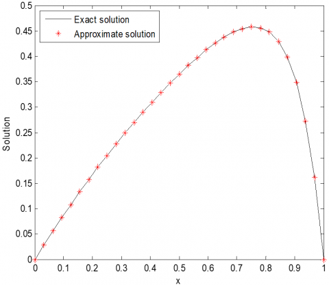
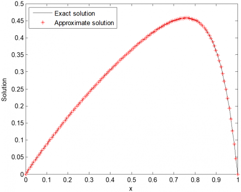
The proposed method provides fourth-order convergence results whenever previous existing methods provide the second-order convergence result. Figures 1 and 2 show the graphical representation of exact and approximate solution.
Example 2: Consider the following two-parameter singularly perturbed boundary value problem from [15, 19, 21, 23].
$-\varepsilon {u}''+\mu {u}'+u=\cos \left( \pi x \right),$$x=\left( 0,\,\,1 \right)$
subject to boundary conditions:
$u\left( 0 \right)=0,\,u\left( 1 \right)=0.$
The exact solution of the example 2 is
$u\left( x \right)=a\,\cos \left( \pi x \right)+b\,\sin \left( \pi x \right)+{{C}_{1}}\,{{e}^{{{\lambda }_{1}}x}}+{{C}_{2}}\,{{e}^{-{{\lambda }_{2}}\left( 1-x \right)}},$
where,
$\begin{align} & a=\frac{\varepsilon {{\pi }^{2}}+1}{{{\mu }^{2}}{{\pi }^{2}}+{{\left( \varepsilon {{\pi }^{2}}+1 \right)}^{2}}},\,\,\,b=\frac{\mu \pi }{{{\mu }^{2}}{{\pi }^{2}}+{{\left( \varepsilon {{\pi }^{2}}+1 \right)}^{2}}}, \\ & {{C}_{1}}=-a\frac{1+{{e}^{-{{\lambda }_{2}}}}}{1-{{e}^{{{\lambda }_{1}}-{{\lambda }_{2}}}}},\,\,\,{{C}_{2}}=a\frac{1+{{e}^{{{\lambda }_{1}}}}}{1-{{e}^{{{\lambda }_{1}}-{{\lambda }_{2}}}}},\,\,\,\,\,{{\lambda }_{1,2}}=\frac{\mu \mp \sqrt{{{\mu }^{2}}+4\varepsilon }}{2\varepsilon }. \\\end{align}$
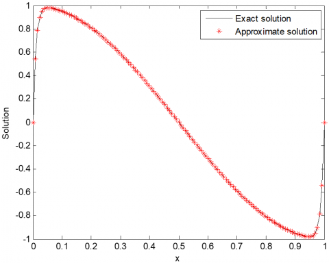
The maximum absolute errors of example 2 are summarized in Tables 3 and 4 at $\varepsilon=10^{-2}, \varepsilon=10^{-4}$ and $N=128$ and different values of $\mu$, respectively. Comparisons with other existing techniques are also mentioned in Tables 3, 4. These tables depicts that the proposed method gives a more accurate approximate solution than the existing methods. This method provides fourth-order convergence results whenever previous existing methods provide the first or second-order convergence result. Figure 3 and 4 are shows the graphical representation of exact and approximate solution.
Figure 1. Graphical representation of exact and approximate solution of example 1 for $\varepsilon=0.1, \mu=1$ and $N=32$
Figure 2. Graphical representation of exact and approximate solution of example 1 for $\varepsilon=0.1, \mu=1$ and $N=32$
Table 3. Comparison of maximum absolute error with other existing methods of example 2 for $\varepsilon=10^{-2}$ and $N=128$
|
$\mu \downarrow$ |
Kadalbajoo and Yadaw [15] |
Zahra and El Mhlawy [21] |
Pandit and Kumar [19] |
Khandelwal and Khan [23] |
Present method |
|
$10^{-3}$ |
8.3832E-05 |
4.1924E-05 |
4.2303E-05 |
6.0243E-06 |
7.2704E-07 |
|
$10^{-4}$ |
8.2686E-05 |
4.1296E-05 |
4.1318E-05) |
6.1827E-07 |
7.3425E-08 |
|
$10^{-5}$ |
8.2572E-05 |
4.1232E-05 |
4.1220E-05 |
1.1455E-07 |
2.6931E-08 |
|
$10^{-6}$ |
8.2561E-05 |
4.1226E-05 |
4.1210E-05 |
7.2269E-08 |
2.4863E-08 |
|
$10^{-7}$ |
8.2560E-05 |
4.1225E-05 |
4.1209E-05 |
6.8266E-08 |
2.4661E-08 |
Figure 3. Graphical representation of exact and approximate solution of example 2 for $\varepsilon=10^{-2}, \mu=10^{-3}$ and $N=128$
Figure 4. Graphical representation of exact and approximate solution of example 2 for $\varepsilon=10^{-4}, \mu=10^{-5}$ and $N=128$
Table 4. Comparison of maximum absolute error with other existing methods of example 2 for $\varepsilon=10^{-4}$ and $N=128$
|
$\mu \downarrow$ |
Kadalbajoo and Yadaw [15] |
Zahra and El Mhlawy [21] |
Pandit and Kumar [19] |
Khandelwal and Khan [23] |
Present method |
|
$10^{-3}$ |
9.4446E-03 |
4.7598E-03 |
5.1964E-03 |
6.2154E-03 |
2.7628E-04 |
|
$10^{-4}$ |
9.0436E-03 |
4.2856E-03 |
4.1710E-03 |
1.8330E-03 |
2.7220E-04 |
|
$10^{-5}$ |
9.0036E-03 |
4.2295E-03 |
4.0754E-03 |
1.1412E-03 |
2.7146E-04 |
|
$10^{-6}$ |
8.9996E-03 |
4.2238E-03 |
4.0659E-03 |
1.3699E-03 |
2.7138E-04 |
|
$10^{-4}$ |
8.9992E-03 |
4.2232E-03 |
4.0650E-03 |
1.3656E-03 |
2.7138E-04 |
In this communication, a fourth order compact finite difference method have studied for numerical solution of two-parameter singularly perturbed convection-diffusion boundary value problems. Present method is computationally efficient. The algorithm of this method is easy to implement on computer and it gives fourth order convergence result. Comparison of the methods are also delineated through Tables 1, 2, 3 and 4 which is indicated that this scheme gives better numerical solution as compared with previously applied techniques with the same mesh point.
The authors wish to express their thanks to the anonymous reviewers for very valuable comments and suggestions, which helped us to improve the quality of the article.
[1] Bigge, J., Bohl, E. (1985). Deformations of the bifurcation diagram due to discretization. Mathematics of Computation, 45: 393-403. https://doi.org/10.1090/S0025-5718-1985-0804931-X
[2] Bohlh, E. (1981). Finite Modele gewohnlicher Randwertaufgaben, Teubner, Stuttgart.
[3] Chen, J., O’Malley, R.E. (1974). On the asymptotic solution of a two-parameter boundary value problem of chemical reactor theory. SIAM Journal of applied Mathematics. 26(4): 717-729. https://doi.org/10.1137/0126064
[4] DiPrima, R. (1968). Asymptotic methods for an infinitely long slider squeeze-film bearing. Journal of Lubrication Technology, 90(1): 173-183. https://doi.org/10.1115/1.3601534
[5] Nayfeh, A.H. (1993). Introduction to Perturbation Techniques, John Wiley and Sons, New York, USA.
[6] Vasileva, A. (1963). Asymptotic methods in the theory of ordinary differential equations containing small parameters in front of the highest derivatives. USSR Computational Mathematics and Mathematical Physics, 3(4): 823-863. https://doi.org/10.1016/0041-5553(63)90381-1
[7] O'Malley, R.E. (1967). Singular perturbations of boundary value problems for linear ordinary differential equations involving two parameters. Journal of Mathematical Analysis and Applications, 19(2): 291-308. https://doi.org/10.1016/0022-247X(67)90124-2
[8] Aziz, T., Khan, A. (2002). A spline method for second-order singularly perturbed boundary-value problems. Journal of Computational and Applied Mathematics, 147(2): 445-452. https://doi.org/10.1016/S0377-0427(02)00479-X
[9] Khan, A., Khandelwal, P. (2014). Non-polynomial sextic spline solution of singularly perturbed boundary-value problems. International Journal of Computer Mathematics, 19(5): 1122-1135. https://doi.org/10.1080/00207160.2013.828865
[10] Khan, A., Khan, I., Aziz, T. (2006). Sextic spline solution of singularly perturbed boundary value problem. Applied Mathematics and Computation, 181(1): 432-439. https://doi.org/10.1016/j.amc.2005.12.059
[11] Lodhi, R.K., Mishra, H.K. (2017). Quintic B-spline method for solving second order linear and nonlinear singularly perturbed two-point boundary value problems. Journal of Computational and Applied Mathematics, 319: 170-187. https://doi.org/10.1016/j.cam.2017.01.011
[12] Brdar, M., Zarin, H. (2016). On a graded meshes for a two-parameter singularly perturbed problem. Applied Mathematics and Computation, 282: 97-107. https://doi.org/10.1016/j.amc.2016.01.060
[13] Gracia, J.L., O’Riordan, E., Pickett, M.L. (2006). A parameter robust second order numerical method for a singularly perturbed two-parameter problem. Applied Numerical Mathematics, 56(7): 962-980. https://doi.org/10.1016/j.apnum.2005.08.002
[14] Kadalbajoo, M.K., Jha, A. (2012). Exponentially fitted cubic spline for two-parameter singularly perturbed boundary value problems. International Journal of Computer Mathematics, 89(6): 836-850. https://doi.org/10.1080/00207160.2012.663492
[15] Kadalbajoo, M.K., Yadaw, A.S. (2008). B-spline collocation method for a two-parameter singularly perturbed convection-diffusion boundary value problems. Applied Mathematics and Computation, 201(1-2): 504-513. https://doi.org/10.1016/j.amc.2007.12.038
[16] Kumar, D., Yadaw, A.S., Kadalbajoo, M.K. (2013). A parameter-uniform method for two-parameter singularly perturbed boundary value problems via asymptotic expansion. Applied Mathematics & Information Science, 7(4): 1525-1532. http://dx.doi.org/10.12785/amis/070436
[17] LinB, T., Roos, H.G. (2004). Analysis of a finite-difference scheme for a singularly perturbed problem with two small parameters. Journal of Mathematical analysis and applications, 289(2): 355-366. https://doi.org/10.1016/j.jmaa.2003.08.017
[18] O’Malley Jr., R.E., (1967). Two-parameter singular perturbation problems for second order equations. Journal of Mathematics and Mechanics, 16(10): 1143-1164.
[19] Pandit, S., Kumar, M. (2014). Haar wavelet approach for numerical solution of two parameters singularly perturbed boundary value problems. Applied Mathematics & Information Science, 8(6): 2965-2974. http://dx.doi.org/10.12785/amis/080634
[20] Valarmathi, S., Ramanujam, N. (2003). Computational method for solving two-parameter singularly perturbed boundary value problems for second-order ordinary differential equations. Applied Mathematics and Computation, 136(2-3): 415-441. https://doi.org/10.1016/S0096-3003(02)00053-X
[21] Zahra, W.K., El Mhlawy, A.M. (2013). Numerical solution of two-parameter singularly perturbed boundary value problems via exponential spline. Journal of King Saud University-Science., 25(3): 201-208. https://doi.org/10.1016/j.jksus.2013.01.003
[22] Shishkin, G.I., Titov, V.A. (1976). A difference scheme for a differential equation with two small parameters multiplying the derivatives, Numer. Method Contin. Medium Mech., 7(2): 145-155.
[23] Khandelwal, P., Khan, A. (2017). Singularly perturbed convection-diffusion boundary value problems with two small parameters using non-polynomial spline technique. Mathematical Sciences, 11: 119-126. https://doi.org/10.1007/s40096-017-0215-3
[24] Miller, J.J.H., O’Riordan, E., Shishkin, G.I. (1996). Fitted numerical methods for singular perturbation problem. World Scientific, Singapore.
[25] O’Malley Jr., R.E. (1974). Introduction to Singular Perturbations, Academic Press, New York.
[26] Lin, B., Li, K., Cheng, Z. (2009). B-spline solution of a singularly perturbed boundary value problem arising in biology. Chaos, Solitions & Fractals, 42(5): 2934-2948. https://doi.org/10.1016/j.chaos.2009.04.036
[27] Henrici, P. (1962). Discrete variable methods in ordinary differential equations. Wiley, New York.