Sergey Ershkov* | Dmytro Leshchenko
© 2021 IIETA. This article is published by IIETA and is licensed under the CC BY 4.0 license (http://creativecommons.org/licenses/by/4.0/).
OPEN ACCESS
We have presented in this analytical research the revisiting of approach for mathematical modeling the Glacier dynamics in terms of viscous-plastic theory of 2-dimensional movements within (x, y)-plane in cartesian coordinates. The stationary creeping approximation for the plane-parallel flow of slowly moving glacial ice on absolutely flat surface without any inclination has been considered. Even in such simple formulation, equations of motion that governs by the dynamics of viscous-plastic flow of glacial ice is hard to be solved analytically. We have succeeded in obtaining analytical expression for the components of velocity in Ox-direction of motion for slowly moving glacial ice (Ox-axis coincides to the initial main direction of slowly moving glacial ice). Restrictions on the form of flow stem from the continuity equation as well as from the special condition for non-Newtonian (viscous-plastic) flow have been used insofar.
basal slip, creeping flow, critical maximal level of stress, glacier dynamics, glacial ice, non-Newtonian fluid, viscous-plastic flow
The glacier is a massive, slowly moving mass of compacted snow and ice. Mainly, the action of gravity governs the dynamics of mass of ice flowing e.g. down the slope side: glaciers are being moved from a one millimeter to hundreds meters (during a day). There are two kinds of motion: 1) a slow sliding motion and an avalanche like flow; 2) the internal movement of glacial ice is a flow similar to plastic flow and viscous flow [1-3]. Glaciers are known to be moving by essentially two mechanisms: Basal slip and viscous-plastic flow. In basal slip, the entire glacier slides over the bed of rock. A glacier’s flow can be also considered as plastic flow, in which it flows as a viscous fluid [4-6].
Illuminating the basic mechanisms, which govern by the dynamics of glaciers, plays a significant role at predicting of tracing of the prescribed trajectory for the entire glacier, moving under the action of non-Newtonian hydrodynamical forces, gradient of pressure and gravity; this is extremely non-linear problem even in the case of glacier’s slow spatial movement in 2D case (in two dimensions) on absolutely flat surface without any inclination. It is worth to note that only a few cases of analytical or semi-analytical solution are known in the field of glacier dynamics [7]; the problem of stability of motion of glacier dynamics or dynamical response to external influence as well as dynamical behavior have been studied in the past under various versions and there is a rich and extended international bibliography [8], especially in recent researches [9-11]. In the current research, we will restrict ourselves in presenting a new analytical technique for revisiting of Glacier dynamics for 2D plane-parallel stationary approximation, by providing the analytical solution for the case of creeping flow [12]. As for the complete introduction to the problem under consideration, we recommend seminal article [7], where a significant historical retrospection has been made as well as all difficulties regarding stability of motion are considered (we mean the appropriate remarks regarding the stability of the solutions and how we are able to study it in the suggested particular problem).
According to Klimov et al. [1] (branch 2.2.2), system of basic equations that governs by the dynamics of viscous-plastic flow of glacial ice should be presented in 2D case in the Cartesian coordinates as below (axis Ox coincides to the initial main direction of slowly moving glacial ice flow on absolutely flat surface without any inclination, z = const; internal dynamics of ice flow is assumed to be corresponding to the simple case of plane-parallel flow, without local intermixing of glacial ice layers, under appropriate boundary conditions):
$\rho\left(\frac{\partial v_{x}}{\partial t}+v_{x} \frac{\partial v_{x}}{\partial x}+v_{y} \frac{\partial v_{x}}{\partial y}\right)=-\frac{\partial p}{\partial x}+\frac{\partial s_{x x}}{\partial x}+\frac{\partial s_{x y}}{\partial y}$,
$\rho\left(\frac{\partial v_{y}}{\partial t}+v_{x} \frac{\partial v_{y}}{\partial x}+v_{y} \frac{\partial v_{y}}{\partial y}\right)=-\frac{\partial p}{\partial y}+\frac{\partial s_{x y}}{\partial x}-\frac{\partial s_{x x}}{\partial y}$,
$\frac{\partial v_{x}}{\partial x}+\frac{\partial v_{y}}{\partial y}=0, U=\sqrt{4\left(\frac{\partial v_{x}}{\partial x}\right)^{2}+\left(\frac{\partial v_{x}}{\partial y}+\frac{\partial v_{y}}{\partial x}\right)^{2}}$, (1)
$s_{x x}=2\left(\mu+\frac{\tau_{s}}{U}\right) \frac{\partial v_{x}}{\partial x}, s_{x y}=2\left(\mu+\frac{\tau_{s}}{U}\right)\left(\frac{\partial v_{x}}{\partial y}+\frac{\partial v_{y}}{\partial x}\right)$,
$\left\{\begin{array}{c}U=\frac{1}{\mu}\left(\sqrt{s_{x x}^{2}+\frac{s_{x y}^{2}}{4}}-\tau_{s}\right), \\ \frac{\partial v_{x}}{\partial x}=s_{x x} / 2\left(\mu+\frac{\tau_{s}}{U}\right),\end{array}\right.$ (2)
where (according to the results of work [1]), ρ is the density of glacial ice; vx is the component of ice velocity in the Ox-direction; vy the component of ice velocity in the Oy-direction; p is the internal pressure (inside the flow of glacial ice); sxx, sxy are the appropriate components of stress tensor; μ is the coefficient of glacial ice dynamic viscosity (which is supposed to be locally constant); τs is a critical maximal level of stress in the shared layer of glacial ice when it begin to move as viscous flow.
Let us consider the case of creeping, plane-parallel flow of glacial ice in (1). Such essential simplification reduces the left part of (1) to be approximately equals to zero due to negligible terms (in the left part) for slowly moving glacial ice with respect to the right part of momentum Eq. (1) (including terms, associated with viscous forces). So, we obtain from (1)-(2):
$0=-\frac{\partial p}{\partial x}+\frac{\partial s_{x x}}{\partial x}+\frac{\partial s_{x y}}{\partial y}$,
$0=-\frac{\partial p}{\partial y}+\frac{\partial s_{x y}}{\partial x}-\frac{\partial s_{x x}}{\partial y}$,
$\frac{\partial v_{x}}{\partial x}+\frac{\partial v_{y}}{\partial y}=0, \frac{\partial v_{x}}{\partial x}=s_{x x} / 2\left(\mu+\frac{\tau_{s}}{U}\right)$,
$U=\frac{1}{\mu}\left(\sqrt{s_{x x}^{2}+\frac{s_{x y}^{2}}{4}}-\tau_{s}\right)$. (3)
Taking into account that p (x, y) = const according to the hydrostatic pressure formula at z = const for the plane-parallel flow of glacial ice, the cross-differentiating of the 1-st and 2-nd equation of (3) in regard to the coordinates x, y yields (we should differentiate 1-st equation of (3) in regard to y, the 2-nd in regard to x, then sum them to each other, p = const).
$\frac{\partial^{2} s_{x y}}{\partial x^{2}}+\frac{\partial^{2} s_{x y}}{\partial y^{2}}=0$ (4)
Eq. (4) means that sxy is the harmonic function [12]; equations of such a type are known to have fundamental solutions as presented below ({x, y} ≠ 0).
$s_{x y} \sim \frac{1}{2 \pi} \ln \left(\sqrt{x^{2}+y^{2}}\right)$ (5)
Taking into account (5), we obtain from Eq. (3)
$\frac{\partial s_{x x}}{\partial x}+\frac{\partial s_{x y}}{\partial y}=0 \Rightarrow s_{x x} \sim-\frac{1}{2 \pi} \arctan \left(\frac{x}{y}\right)+f(y)$ (6)
where, f(y) is the arbitrary function, depending on y, which should be determined from the second of Eq. (3) and Eqns. (5)-(6) as below
$\frac{\partial s_{x y}}{\partial x}-\frac{\partial s_{x x}}{\partial y}=0$
$\left\{\frac{\partial s_{x x}}{\partial y} \sim \frac{x}{2 \pi}\left(\frac{1}{1+\left(\frac{x}{y}\right)^{2}}\right) \frac{1}{y^{2}}+\frac{d f(y)}{d y}\right\} \Rightarrow$
$\frac{1}{2 \pi}\left(\frac{x}{\left(x^{2}+y^{2}\right)}\right)-\left\{\frac{x}{2 \pi}\left(\frac{1}{1+\left(\frac{x}{y}\right)^{2}}\right) \frac{1}{y^{2}}+\frac{d f(y)}{d y}\right\}=0$
$\Rightarrow \frac{d f(y)}{d y}=0$ (7)
so, we can conclude from (7) that f(y) = C = const.
Let us present the exact solution for the components of velocity field in case of creeping, plane-parallel flow of glacial ice. We can obtain from (3) as below:
$\frac{\partial v_{x}}{\partial x}=\frac{s_{x x}}{2 \mu}\left(1-\frac{\tau_{s}}{\sqrt{s_{x x}^{2}+\frac{s_{x y}^{2}}{4}}}\right), \Rightarrow$
$\frac{\partial v_{x}}{\partial x}=\frac{\left(C-\frac{1}{2 \pi} \arctan \left(\frac{x}{y}\right)\right)}{2 \mu}$
$\left(1-\frac{\tau_{s}}{\sqrt{\left(C-\frac{1}{2 \pi} \arctan \left(\frac{x}{y}\right)\right)^{2}+\frac{\left(\frac{1}{2 \pi} \ln \left(\sqrt{x^{2}+y^{2}}\right)\right)^{2}}{4}}}\right)$
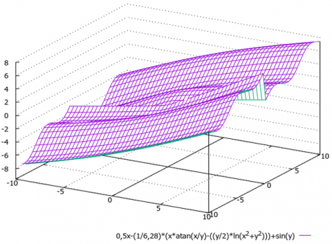
where we can assume just for simplicity τs $\cong$0; so, we should obtain the expression for component vx as shown below (we imagine also the plot of component vx at Figure 1):
$\frac{\partial v_{x}}{\partial x}=\frac{\left(C-\frac{1}{2 \pi} \arctan \left(\frac{x}{y}\right)\right)}{2 \mu}, \Rightarrow$
$\Rightarrow v_{x}=\frac{1}{2 \mu}\left(C x-\frac{1}{2 \pi}\left[\begin{array}{l}x \arctan \left(\frac{x}{y}\right) \\ -\frac{y}{2} \ln \left(x^{2}+y^{2}\right)\end{array}\right]\right)+g(y)$ (8)
Taking also into consideration the continuity equation in (3) and Eq. (8), we could obtain the expression for component vy:
$v_{y}=\frac{1}{2 \mu}\left(\frac{x}{2 \pi} \int\left(\arctan \left(\frac{1}{u}\right)\right) d u-C y\right)$
$+h(x),\left\{u=\left(\frac{y}{x}\right)\right\}$ (9)
We should additionally take into account the appropriate equation in Eq. (3) for the component of stress tensor sxy which stems in unchanged form from Eq. (1) (where by restricting in choosing of the functions g (y), h (x) we should satisfy both the parts of such the equation; here and below we will assume τs $\cong$ 0 as mentioned above, glacial ice moves as viscous flow of non-Newtonian fluid):
$s_{x y}=2\left(\mu+\frac{\tau_{s}}{U}\right)\left(\frac{\partial v_{x}}{\partial y}+\frac{\partial v_{y}}{\partial x}\right)$,
$\left\{U=\frac{1}{\mu}\left(\sqrt{s_{x x}^{2}+\frac{s_{x y}^{2}}{4}}-\tau_{s}\right)\right\}$,
$\Rightarrow s_{x y}\left(1-\frac{\tau_{s}}{\sqrt{s_{x x}{ }^{2}+\frac{s_{x y}{ }^{2}}{4}}}\right)=2 \mu\left(\frac{\partial v_{x}}{\partial y}+\frac{\partial v_{y}}{\partial x}\right)$,
$\Rightarrow s_{x y} \cong 2 \mu\left(\frac{\partial v_{x}}{\partial y}+\frac{\partial v_{y}}{\partial x}\right)$,
$\Rightarrow \frac{1}{2 \pi} \ln \left(\sqrt{x^{2}+y^{2}}\right)=2 \mu\left(\frac{\partial v_{x}}{\partial y}+\frac{\partial v_{y}}{\partial x}\right)$,
$v_{x}=\frac{1}{2 \mu}\left(C x-\frac{1}{2 \pi}\left[\begin{array}{c}x \arctan \left(\frac{x}{y}\right) \\ -\frac{y}{2} \ln \left(x^{2}+y^{2}\right)\end{array}\right]\right)+g(y)$,
$v_{y}=\frac{1}{2 \mu}\left(\frac{x}{2 \pi} \int\left(\arctan \left(\frac{1}{u}\right)\right) d u-C y\right)$
$+h(x),\left\{u=\left(\frac{y}{x}\right)\right\}$ (10)
As we can see, Eq. (10) above could obviously be solved by numerical methods only or by appropriate approximation technique e.g. by the series of Taylor expansions [12] (for the appropriate boundary conditions).
Figure 1. A schematic plot of the function vx = vx(x,y)
Figure 1 let us conclude that such the schematical presenting of analytical solutions seems to be the only way to get some kind of information about the intrinsic properties and behavior of the particular dynamical system, depending on the chosen initial or boundary conditions (on Figure 1 meanings of function vx = vx(x,y) is on vertical axis, meanings of {x,y} are scaled for each coordinate with respect to the appropriate horizontal axis).
Let us discuss our novel approach and results in obtaining a new class of exact solutions for the components of velocity field in case of creeping, plane-parallel flow of glacial ice. First, we should discuss the basic approach, suggested by Klimov et al. [1] (the main reason that our partial solving procedure is based on their constitutive modeling approach to a visco-plastic fluid). According to aforementioned ansatz, nonstationary flow of a viscoelastic medium between two parallel plates was considered in ref. [1] for the case of a varying pressure gradient. The problem was reduced to the Stephan problem, with the condition on the boundary separating the flow domain from the quasi-rigid domain. Four multiparameter families of exact solutions were found by Klimov et al. [1]. The first family describes the flow decelerations up to a full stop. The second family determines the development of the flow from the state of rest as the pressure gradient increases. The third family describes the development of the flow for the case where (1) the pressure gradient is constant and exceeds the threshold value related to the yield stress, (2) the upper boundary plate does not move, and (3) the lower boundary plate moves with a constant acceleration. Finally, the fourth family determines the flow retardation, when the pressure gradient is constant and is less than the threshold value.
The solution, obtained in the current research, corresponds to the simple case of absence of pressure gradient (the constant internal pressure inside the flow of glacial ice, according to the hydrostatic pressure formula at z = const for the plane-parallel flow of glacial ice) for glacier’s slow or creeping spatial movement in two dimensions on absolutely flat surface without any inclination. It allows us to reduce the general formulation of the problem in a form (1)-(2) to the simplest form (3) which then can be successfully integrated by means of analytical methods via cross-differentiating of the 1-st and 2-nd equation of (3) in regard to the coordinates {x, y}, taking into account continuity equation as well. As a result, we obtain the Laplace Eq. (4) (in regard to component of stress tensor sxy) and, thus, we come to conclusion that component of stress tensor sxy should be presented by the harmonic function in a form (5), depending on spatial coordinates {x, y}. Using (5), we obtain further the appropriate expressions (6)-(7) from the equations of motion (3) for the component of stress tensor sxx, which should satisfy all the aforementioned equations. So, we can obtain the proper analytical formulae (8)-(9) from (2) for the components of velocity field {vx, vy} (choosing those that satisfy continuity equation) with arbitrary functions g (y), h (x).
Such arbitrary functions g (y), h (x) should satisfy both the parts of Eq. (10) (which also stems from presentation of the problem (2)) under the appropriate boundary conditions, whereas aforementioned Eq. (10) could obviously be solved by numerical methods only or by appropriate approximation technique e.g. by the series of Taylor expansions. We present the schematical plot (Figure 1) imaging the solution for component of velocity field vx (for the case of special choice of the boundary conditions).
Finalizing discussion, we should especially note that, as we can see from discussion above, system of equations (which governs by the dynamics of viscous-plastic flow of glacial ice) is hard to solve analytically even in case of slowly moving glacial ice flow on absolutely flat surface without any inclination. To the best of our knowledge, analytical solutions for the general case do not exist. So, any new theoretical method or approach for even the particular solving of the aforementioned system of equations would be useful on the level of practical applications. We guess that description with respect of the gained analytical results (presented here) is enough for specialists in hydrodynamics to gain a new insight regarding possible glacial ice’s flat movements without any inclination.
The last but not least, let us consider further and below the 2D case of creeping, nonstationary flow of glacial ice which stems from (1)-(2) (as for the basic equations for 3D gravity-driven flow of glacial ice, see Appendix).
Such essential simplification reduces convective terms in the left part of (1) to be approximately equals to zero due to presence there the negligible terms (for slowly moving glacial ice) with respect to the right part of momentum Eq. (1) (mainly, to the terms, associated with viscous forces). So, we obtain from (1)-(2):
$\left\{\begin{array}{l}\rho \frac{\partial v_{x}}{\partial t}=-\frac{\partial p}{\partial x}+2 \mu\left(\frac{\partial^{2} v_{x}}{\partial x^{2}}+\frac{\partial^{2} v_{y}}{\partial x \partial y}+\frac{\partial^{2} v_{x}}{\partial y^{2}}\right), \\ \rho \frac{\partial v_{y}}{\partial t}=-\frac{\partial p}{\partial y}-2 \mu\left(\frac{\partial}{\partial y}\left(\frac{\partial v_{y}}{\partial y}+\frac{\partial v_{x}}{\partial x}\right)\right) \\ +2 \mu \frac{\partial^{2} v_{y}}{\partial x^{2}}, \frac{\partial v_{x}}{\partial x}+\frac{\partial v_{y}}{\partial y}=0,\end{array}\right.$
$\Rightarrow\left\{\begin{array}{l}\rho \frac{\partial v_{x}}{\partial t}=-\frac{\partial p}{\partial x}+2 \mu \frac{\partial^{2} v_{x}}{\partial y^{2}}, \\ \rho \frac{\partial v_{y}}{\partial t}=-\frac{\partial p}{\partial y}+2 \mu \frac{\partial^{2} v_{y}}{\partial x^{2}}, \\ \frac{\partial v_{x}}{\partial x}+\frac{\partial v_{y}}{\partial y}=0,\end{array}\right.$ (11)
where, we also have assumed τs @ 0 just for simplicity in the shared layer (so, glacial ice permanently moves as viscous flow of non-Newtonian fluid).
We should note that 1st and 2nd equations of system (11) are known to have appropriate solutions as 1-dimensional heat equation [12] with respect to the chosen coordinate y (first equation) or x (second equation), which nevertheless should be ajusted to each other by additionally using of the 3rd, continuity equation. E.g., such the ajusting can be made by using the proper invariant below:
$0=-\frac{\partial^{2} p}{\partial x^{2}}-\frac{\partial^{2} p}{\partial y^{2}}+2 \mu \frac{\partial^{2}}{\partial y^{2}}\left(\frac{\partial v_{x}}{\partial x}\right)+2 \mu \frac{\partial^{2}}{\partial x^{2}}\left(\frac{\partial v_{y}}{\partial y}\right), \Rightarrow$
$\Rightarrow\left\{\frac{\partial v_{x}}{\partial x}+\frac{\partial v_{y}}{\partial y}=0\right\} \Rightarrow \frac{\partial^{2}}{\partial x^{2}}\left(\frac{\partial v_{x}}{\partial x}\right)-\frac{\partial^{2}}{\partial y^{2}}\left(\frac{\partial v_{x}}{\partial x}\right)=-\frac{\Delta p}{2 \mu}$.
But since at this stage algorithm for further obtaining of exact solution has no chance to be presented in analytical or semi-analytical way, we should apply additional simplifications to equations of system (11):
$\Rightarrow\left\{\begin{array}{l}\frac{\partial v_{x}}{\partial x}+\frac{\partial v_{y}}{\partial y}=0 \\ \frac{\partial^{3} v_{x}}{\partial y^{3}}=\frac{\partial^{3} v_{y}}{\partial x^{3}}, \Rightarrow \\ \frac{\partial p}{\partial x}=2 \mu \frac{\partial^{2} v_{x}}{\partial y^{2}}\end{array}\right. \left\{\begin{array}{l}\frac{\partial^{4} v_{x}}{\partial x^{4}}+\frac{\partial^{4} v_{x}}{\partial y^{4}}=0, \\ \frac{\partial v_{y}}{\partial y}=-\frac{\partial v_{x}}{\partial x}, \\ \frac{\partial p}{\partial x}=2 \mu \frac{\partial^{2} v_{x}}{\partial y^{2}}\end{array}\right.$ (12)
$\left\{\begin{array}{l}\rho \frac{\partial v_{x}}{\partial t}=2 \mu \frac{\partial^{2} v_{x}}{\partial y^{2}}, \\ \rho \frac{\partial v_{y}}{\partial t}=2 \mu \frac{\partial^{2} v_{y}}{\partial x^{2}}, \Rightarrow \\ \frac{\partial v_{x}}{\partial x}+\frac{\partial v_{y}}{\partial y}=0,\end{array}\right.$
$\left\{\begin{array}{c}v_{x}=\frac{1}{\sqrt{4 \pi\left(\frac{2 \mu}{\rho}\right) t}} \exp \left(-\frac{y^{2}}{4\left(\frac{2 \mu}{\rho}\right) t}\right), \\ v_{y}=\frac{1}{\sqrt{4 \pi\left(\frac{2 \mu}{\rho}\right) t}} \exp \left(-\frac{x^{2}}{4\left(\frac{2 \mu}{\rho}\right) t}\right), \\ \frac{\partial v_{x}}{\partial x}+\frac{\partial v_{y}}{\partial y}=0,\end{array}\right.$ (13)
Thus, we have pointed out two additional classes of exact solutions (12)-(13) of Eqns. (1)-(2) in their approximation (11) for creeping flow of glacial ice, which differ from solutions (10) for stationary approximation creeping flow of glacial ice with constant pressure field along the path of the plane-parallel flow of glacial ice. Videlicet, 1st class is also associated with stationary flow (but variable pressure field), the 2nd stems from assumption of constant pressure field along the path of the plane-parallel flow, but we have considered nonstationary case of glacial ice in this case.
As for the purpose of current research reported in this paper, we can formulate it as follows: the main aim is to find a kind of exact solution to the system of Eq. (3) under consideration. Namely, each exact solution can clarify the structure, intrinsic code and topology of the variety of possible solutions (from mathematical point of view).
As we can see from derivation presented above in Sections 2-3, system of Eq. (1) that governs by the dynamics of viscous-plastic flow of glacial ice is unlikely to be solved analytically in general case.
Indeed, we have explored here the conditions for analytical solving the reduced version (3) of the aforementioned system (1) of equations for 2D plane-parallel stationary approximation of creeping flow of slowly moving glacial ice on absolutely flat surface without any inclination. Even in this simple case, we woud need the semi-analytical approximation for pointing out the appropriate expressions for functions g(y), h (x) in (8)-(10) (according to the boundary conditions).
Let us list below the obvious assumptions (or simplifications) which have been used at the formulation or the solution of the problem:
-the assumption of 2D stationary creeping approximation for the flow of glacial ice was used (it means that the inertial forces are preferably ignored in basic momentum equation (1));
-simple case of plane-parallel flow of slowly moving glacial ice on absolutely flat surface without any inclination, without local intermixing of glacial ice layers has been considered (it means pressure p (x, y) = const locally along the path of one layer of glacial ice);
-the coefficient of glacial ice dynamic viscosity μ is supposed to be locally constant;
- distances between various points inside the flows of glacial ice are supposed not to be elongated significantly (continuity equation was used);
-the critical maximal level of stress τs $\cong$0 (is approximately zero) in the shared layer (so, glacial ice permanently moves as viscous flow of non-Newtonian fluid);
-we consider only the Cauchy problem in the whole space (besides, flows of glacial ice is considered to be at rest at infinity).
The last but not least, it is worth to note regarding we can see from the aforementioned list of simplifications that the real conditions for spatial dynamics of glacial ice (e.g., dynamics of arctic Glaciers) are definitely very far from the ideal formulation of what can be solved analytically based on the equations of motion for the glacier’s dynamics. As for developing the main idea, the suggested approach can be used in the future researches for analysis of the surging glaciers [7], not only in simple case of 2D stationary creeping approximation plane-parallel flow (сcompared with reference [7], the linear boundary value problem of the stress tensor field S = {sxx, sxy} in the glacier is considered in the current research). Indeed, predicting of regimes of chaotically forced oscillations inside the huge mass of Glaciers is very useful for problems of providing safety at mountain area.
Also, remarkable works [13-21] should be cited, which concern the problem under consideration.
Authors are thankful to unknown esteemed Reviewer with respect to his valuable efforts and advice which have improved structure of the article significantly.
Remark regarding contributions of authors as below:
In this research, Dr. Sergey Ershkov is responsible for the general ansatz and the solving procedure, simple algebra manipulations, calculations, results of the article in Sections 1-4, and also is responsible for the search of approximated solutions.
Dr. Dmytro Leshchenko is responsible for theoretical investigations as well as for the deep survey in literature on the problem under consideration.
Both authors agreed with results and conclusions of each other in Sections 1-5.
|
v |
velocity of ice flow, m.s-1 |
|
p |
internal pressure, Pa |
|
s |
component of stress tensor, Pa |
|
Greek symbols |
|
|
ρ |
the density of glacial ice, kg. m-3 |
|
µ |
dynamic viscosity, kg. m-1.s-1 |
|
τ |
critical level of stress, Pa |
|
Subscripts |
|
|
x, y, z |
components of ice flow velocity in the Ox, Oy, Oz-directions |
|
xx, yy, zz |
components of stress tensor |
|
s |
critical maximal level of stress in the shared layer of glacial ice |
Let us consider the generalization of Eqns. (1)-(2) for 3D gravity-driven flow of glacial ice (in absolute Cartesian coordinate system):
$\rho\left(\frac{\partial v_{x}}{\partial t}+v_{x} \frac{\partial v_{x}}{\partial x}+v_{y} \frac{\partial v_{x}}{\partial y}+v_{z} \frac{\partial v_{x}}{\partial z}\right)$
$=-\frac{\partial p}{\partial x}+\frac{\partial s_{x x}}{\partial x}+\frac{\partial s_{x y}}{\partial y}+\frac{\partial s_{x z}}{\partial z}+\rho g_{x}$,
$\rho\left(\frac{\partial v_{y}}{\partial t}+v_{x} \frac{\partial v_{y}}{\partial x}+v_{y} \frac{\partial v_{y}}{\partial y}+v_{z} \frac{\partial v_{y}}{\partial z}\right)$
$=-\frac{\partial p}{\partial y}+\frac{\partial s_{y x}}{\partial x}+\frac{\partial s_{y y}}{\partial y}+\frac{\partial s_{y z}}{\partial z}+\rho g_{y}$ (A.1)
$\rho\left(\frac{\partial v_{z}}{\partial t}+v_{x} \frac{\partial v_{z}}{\partial x}+v_{y} \frac{\partial v_{z}}{\partial y}+v_{z} \frac{\partial v_{z}}{\partial z}\right)$
$=-\frac{\partial p}{\partial z}+\frac{\partial s_{z x}}{\partial x}+\frac{\partial s_{z y}}{\partial y}+\frac{\partial s_{z z}}{\partial z}+\rho g_{z}$,
$\frac{\partial v_{x}}{\partial x}+\frac{\partial v_{y}}{\partial y}+\frac{\partial v_{z}}{\partial z}=0, U$
$=\sqrt{2\left(v_{x x}^{2}+v_{y y}^{2}+v_{z z}^{2}\right)+4\left(v_{x y}^{2}+v_{x z}^{2}+v_{y z}^{2}\right)}$,
$s_{i j}=2\left(\mu+\frac{\tau_{s}}{U}\right) v_{i j}, \quad(i, j=\{x, y, z\}) \quad v_{x x}$
$=\frac{\partial v_{x}}{\partial x}, \quad v_{y y}=\frac{\partial v_{y}}{\partial y}, \quad v_{z z}=\frac{\partial v_{z}}{\partial z}$,
$v_{x y}=\frac{1}{2}\left(\frac{\partial v_{x}}{\partial y}+\frac{\partial v_{y}}{\partial x}\right), \quad v_{x z}$
$=\frac{1}{2}\left(\frac{\partial v_{x}}{\partial z}+\frac{\partial v_{z}}{\partial x}\right), \quad v_{y z}=\frac{1}{2}\left(\frac{\partial v_{y}}{\partial z}+\frac{\partial v_{z}}{\partial y}\right)$
[1] Klimov, D.M., Petrov, A.G., Georgievsky, D.V. (2005). Viscous-plastic flows: Dynamical chaos, stability, and confusion. Moscow, Science [in Russian]. https://urait.ru/viewer/mehanika-sploshnoy-sredy-vyazkoplasticheskie-techeniya-426470#page/4.
[2] van der Veen, C.J. (2013). Fundamentals of Glacier Dynamics. CRC Press, 2nd Edition in 2017. https://www.routledge.com/Fundamentals-of-Glacier-Dynamics/Veen/p/book/9781138077218.
[3] Greve, R. (2010). Dynamics of Ice Sheets and Glaciers. Lecture Notes, Sapporo, Institute of Low Temperature Science, Hokkaido University, Japan. https://ocw.hokudai.ac.jp/wp-content/uploads/2016/02/DynamicsOfIce-2005-Note-all.pdf.
[4] Greve, R., Blatter, H. (2009). Dynamics of Ice Sheets and Glaciers. Springer, Berlin, Germany. https://www.springer.com/gp/book/9783642034145.
[5] Hooke, R.L. (2005). Principles of Glacier Mechanics, Cambridge University Press, Cambridge, UK and New York, NY, USA, 2nd edition.
[6] Paterson, W.S.B. (1994). The Physics of Glaciers. Pergamon Press, Oxford, UK etc., 3rd edition.
[7] Halfar, P. (2020). Surging glaciers II: mathematically exact two-dimensional stress tensor fields. Acta Mechanica, 231: 843-856. https://doi.org/10.1007/s00707-020-02615-9
[8] Nick, F.M., Vieli, A., Howat, I.M., Joughin, I. (2009). Large-scale changes in Greenland outlet glacier dynamics triggered at the terminus. Nature Geoscience, 2: 110-114. https://doi.org/10.1038/ngeo394
[9] Wu, Z., Zhang, H., Liu, S., Ren, D., Bai, X., Xun, Z., Ma, Z. (2019). Fluctuation analysis in the dynamic characteristics of continental glacier based on Full-Stokes model. Scientific Reports, 9(1): 1-17. https://doi.org/10.1038/s41598-019-56864-3
[10] Williams, J.J., Gourmelen, N., Nienow, P. (2020). Dynamic response of the Greenland ice sheet to recent cooling. Scientific Reports, 10(1): 1-11. https://doi.org/10.1038/s41598-020-58355-2
[11] Kumar, O., Ramanathan, A.L., Bakke, J., Kotlia, B.S., Shrivastava, J.P. (2020). Disentangling source of moisture driving glacier dynamics and identification of 8.2 ka event: Evidence from pore water isotopes, Western Himalaya. Scientific Reports, 10(1): 1-10. https://doi.org/10.1038/s41598-020-71686-4
[12] Ershkov S.V. (2017). Non-stationary creeping flows for incompressible 3D Navier–Stokes equations. European Journal of Mechanics, B/Fluids, 61(1): 154-159. https://doi.org/10.1016/j.euromechflu.2016.09.021
[13] Van der Veen, C.G., Oerlemans, J. (1985). Dynamics of the West Antarctic ice sheet. Proceedings of a Workshop held in Utrecht, May 6-8, Published by D. Reidel Publishinh Company, Dordrecht, Golland.
[14] Åström, J.A., Riikilä, T.I., Tallinen, T., Zwinger, T., Benn, D., Moore, J.C., Timonen J. (2013). A particle based simulation model for glacier dynamics. The Cryosphere, 7(5): 1591-1602. https://doi.org/10.5194/tc-7-1591-2013
[15] Haeberli, W., Hallet, B., Arenson, L., Elconin, R., Humlum, O., Kääb, A., Kaufmann, V., Ladanyi, B., Matsuoka, N., Springman, S., Von der Mühl, D. (2006). Permafrost creep and rock glacier dynamics. Permafrost and Periglacial Processes, 17(3): 189-214. https://doi.org/10.1002/ppp.561
[16] Jiskoot, H. (2011). Dynamics of Glaciers. In: Singh V.P., Singh P., Haritashya U.K. (eds), Encyclopedia of Snow, Ice and Glaciers, Encyclopedia of Earth Sciences Series, Springer, Dordrecht.
[17] Hofmann, F.M., Rauscher, F., McCreary, W., Bischoff, J.P., Preusser F. (2020). Revisiting Late Pleistocene glacier dynamics north-west of the Feldberg, southern Black Forest, Germany. E&G Quaternary Science Journal, 69(1): 61-87. https://doi.org/10.5194/egqsj-69-61-2020
[18] Baaijens, F.P.T. (1998). Mixed finite element methods for viscoelastic flow analysis: A review. Journal of Non-Newtonian Fluid Mechanics, 79(2-3): 361-385. https://doi.org/10.1016/S0377-0257(98)00122-0
[19] Hunke, E.C., Dukowicz, J.K. (1997). An elastic–viscous–plastic model for sea ice dynamics. Journal of Physical Oceanography, 27(9): 1849-1867. https://doi.org/10.1175/1520-0485(1997)027<1849:AEVPMF>2.0.CO;2
[20] Sundal, A.V., Shepherd, A., Van Den Broeke, M., Van Angelen, J., Gourmelen, N., Park, J. (2013). Controls on short-term variations in Greenland glacier dynamics. Journal of Glaciology, 59(217): 883-892. https://doi.org/10.3189/2013JoG13J019
[21] Duval, P., Montagnat, M., Grennerat, F., Weiss, J., Meyssonnier, J., Philip, A. (2010). Creep and plasticity of glacier ice: A material science perspective. Journal of Glaciology, 56(200): 1059-1068. https://doi.org/10.3189/002214311796406185