Rysbek Baimakhan* | Zhanar Kadirova | Assima Seinassinova | Aigerim Baimakhan | Zukhra Abdiakhmetova
© 2021 IIETA. This article is published by IIETA and is licensed under the CC BY 4.0 license (http://creativecommons.org/licenses/by/4.0/).
OPEN ACCESS
The purpose of this article is to present the developed methodology, a brief algorithm of mechanical-and-mathematical modeling to investigate the causes and mechanism of soil disruption from the hillsides and the results of its use for restoring the pre-landslide stress state using the example of one of the tragic landslides. The numerical finite element algorithm of studying the stress–strain state (SSS) of soil deposits of slopes of the inclined-layered structure is briefly described, with specific features of the use of isoparametric elements of the quadrangular shape with four nodes of arbitrary shape. For detailed studying the SSS, the cover soils of the steep slope of the inclined-layered structure, in height from the arch to the foot, are conventionally divided into three zones, each of which has layered structures. Studies of the geometry of its area and the angle of inclination of the slope showed that the two-layer structure of its original structure made a curved path repeating the outline of the gorge. The finite element method helped to model the soil deposits of the slope with the granite-basalt rock as close as possible to the landslide initial shape. The proposed methodology, the mechanical-mathematical model, algorithms and calculation examples allow predicting the possible occurrence of landslides on other countless hillsides of the Northern Tien Shan by determining stress concentration zones.
hillside, inclined layers, landslide, soil, stress
The main cause of landslides on hillsides is the process of infiltration that is associated with penetration of rain and snow water into inclined soil layers. The layers differ from each other not only in composition and structure but also in physical, mechanical and strength properties. The main volume of rainwater flows down the inclined surface of the soil, some of them evaporate. At the same time, depending on the density and fracture of the surface layer, a certain part of water penetrates into the soil and causes water saturation and soil moisture. This is a long and slow process. When such local zones are joined, a litter is formed that contributes to the soil mass displacement along the slope. Water penetrates the ground through weak points of coupling, cohesive forces between particles. Visual surveys of the tracks of the landslides ‘Ak Kain’, ‘Shym Bulak’, ‘Kok Tobe’, ‘Kol Sai’ show that not one of them has a rocky surface on exposed surfaces after the landslide. Therefore, landslides represent the sliding of rock masses along the water-resistant waterproof layer, arising under the effect of gravity.
Depending on the location, the soil structure, the slope angle, porosity, water saturation, physical-and-mechanical and strength properties, the disruption mechanisms of a part of the soil mass on the hillsides are very diverse. For example, mountain slopes are distinguished by the following formations.
Alluvial deposits on slopes are deposits of water flows that make up river floodplains and terraces and consist of rounded detrital material, such as pebbles, gravel, sands, loams and clays [1], as a result of which erosion processes occur [2]. There are slopes on which the movement of material down the slope occurs as a result of the runoff of rain or melt water in the form of thin intertwining streams covering the entire surface of the slopes with a dense network, they are called deluvial. The deluvium is most often represented by loam or sandy loam [3]. There are also colluvial slope collapses by type. If the size of the debris has a volume of more than 10 m³, the process is called caving, if smaller, it is crumbling. Such caving and crumbling predominate on slopes, the steepness of which is greater than the steepness of the natural slope (35-37°), which is characteristic of the foothill slopes of the Zailiysk Alatau Mountains. Colluvial collapses have repeatedly occurred on the mountain road between the Shym Bulak sports complex and the Medeu high-mountain dam. The last massive collapse on this road occurred after the departure of the then President of Kazakhstan N. Nazarbayev from the sports complex in 2017 [4]. Proluvial collapses have repeatedly occurred on the mountain slopes of the Northern Tien Shan, near the Ak Kain sanatorium. The largest one took place the slopes of the Camel mountain in 2005. Proluvium is loose deposits of rock destruction products washed away and carried along hollows (erosional furrows) by temporary streams from atmospheric precipitation to the foothills of elevations (mountains) [5].
Therefore, the methods, models and approaches for studying landslides on mountain slopes are constantly being improved. For example, Longoni et al. [6] draw attention to the validity of the physical landslide model in calculations using a numerical model, which requires the combination of several surface and underground surveys to achieve a satisfactory spatial resolution. This kind of the model is difficult for practical use. Attention should be paid to two specific aspects: the degree of the model and the accuracy of the input data sets. Brunetti et al [7], to predict landslides of precipitation, proposed the use of so-called satellite rain products. But at the same time, they emphasize the very limited nature of such satellite data today.
Some Indian scientists pay attention to the influence of nearby geological faults on the occurrence of landslides on mountain slopes. Mohit Kumar, Shruti Rana, and others analyzed stability of the ravine on the banks of the Baliya-Nala River, which flows from Lake Nainital in India [8]. The terrain is crossed by geological faults. The effects of the joints and fault zones of faults on stability states of the ravine were studied.
Chinese scientists Kun-Ting Chen and Jian-Hong Wu studied the causes and main dynamic characteristics of the landslide that occurred in the village of Xinmo Diexi, Sichuan, China, June 24, 2017 [9]. Field studies revealed that one of the main causes of increasing the volume of landslides was ablation. To reproduce the behavior of the landslide flow, a continual model averaged over the depth was used, which allowed taking into account the captured soil mass.
Ran et al. [10] studied the landslide infiltration of rainwater water applications, the so-called integrated hydrological model InHM. This model is used in conjunction with the model of infinite slope stability. The last assumption is of course conditional.
Some issues of the model of ultimate equilibrium are considered in work [11]. It shows that the volume of the moving mass decreases with increasing the angle of inclination for given material strength.
Malaysian researchers, Nordiana et al. [12], using the 2D resistivity method, were able to determine the structure of the slope layer in the Selangor of Malaysia. It turns out that the soils of this slope are formed of sand with boulders. Therefore, from the point of view of stability, the ground mass of this slope has reduced strength. A review of the domestic and foreign works on this topic shows the absence of anisotropic, at the same time inclined-layered structure models.
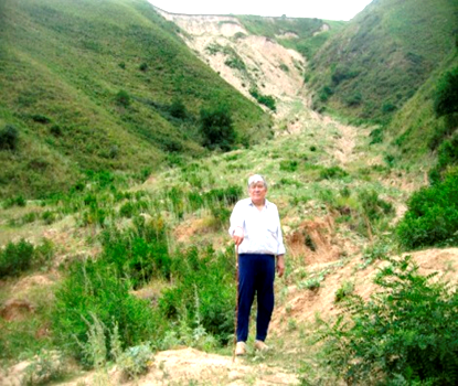
Piedmont slopes of the Northern Tien Shan also have peculiar structures. In early spring 2004, long rainy days began in the Almaty region. On the night of March 14, at 2:15 in the east of the city of Almaty, in the village of Taldybulak, on the slopes of one of the hills near the Ak Bulak sanatorium, the process of sudden displacement of the rock mass began at a high speed. Down the slope there were outbuildings, office space, a residential building. There died all the residents of the two-story residential building. Figure 1 show photographs of one of the authors visual inspection of the landslide ‘Ak Kain’ in place and an enlarged view of the starting point of the tear from the slope wall.
Due to the intense melting of glaciers and more frequent precipitation, many slopes of the foothill hills are in a pre-landslide state.
(a) Studying the landslide in place by the authors
(b) Enlarged photo of the soil mass disruption
Figure 1. Ak Kain landslide in the Northern Tien Shan
At the foot of such slopes there are numerous buildings such as motels, rest houses, sports. Due to the intense melting of glaciers and the frequent precipitation, many slopes of the foothills are in the pre-landslide state.
A visual inspection of the remains of the landslide ‘Ak Kain’ shows that the slope soils are mainly formed by varieties of loams with mixtures of sandy and loamy soils. As it can be seen from right Figure 1, the surface soils of the slope in a large scale consist of two layers of anisotropic structure.
For predictive determination of the pre-landslide state of similar numerous slopes of the Northern Tien Shan and for the adoption of a safety measure to strengthen the slopes of such populated hillsides, a mechanical-and-mathematical calculation model of the hillside of the inclined-layered anisotropic structure is proposed and its implementation using the example of reconstructing the stress–strain state (SSS) picture of the pre-landslide state of the Ak Kain slope.
2.1 Mechanical-mathematical simulation algorithm for the slope SSS
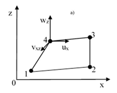
Below there are given some defining basic mathematical functions of a four-node isoparametric element [13]. Figure 2 shows a typical four-node isoparametric finite element of an arbitrary shape (2a) in the Cartesian coordinate system and its representation in the unit coordinate system ξOη (2b).
(a) In the Cartesian coordinate system
(b) In the local coordinate system
Figure 2. Nonlinear isoparametric quadrinodal elements of arbitrary shape
In the FEM strain components are determined by the Cauchy equations in the form:
$\varepsilon_{x}=\frac{\partial u}{\partial x}, \varepsilon_{y}=\frac{\delta \vartheta}{\delta y}$ (1)
$\gamma_{x y}=\frac{\partial \vartheta}{\delta x}+\frac{\partial u}{\partial y}$ (2)
Regardless of the isotropy or anisotropy of the medium, the Martin form of writing the Cauchy equations in the FEM has form (1). The difference is in the matrix of elastic characteristics [D]. For an isotropic medium, the elements of this matrix are determined by the elastic constants E, the Young modulus and ν, the Poisson ratio. For an anisotropic medium, their elements are determined by five elastic constants: two elastic moduli: E1, E2, shear modulus G2 and deformation coefficients -ν1 and ν2.
In the short matrix form, expression (1-2) can be written in the form:
$\{\varepsilon\}_{i, j}=[B]_{i, j}\{U\}$ (3)
where, [B]i,j is the matrix of basic functions which element are calculated at the integration points i and j, and {U} is the vector of displacements.
For the soil of isotropic structure:
Now let’s write down an expression for calculating stress components of the internal integration points i and j:
$\left\{\sigma_{i j}\right\}=[D]\left\{\varepsilon_{i j}\right\}$ (4)
In the last expression:
$\left\{\sigma_{i j}\right\}^{T}=\left\{\sigma_{x_{i j}}, \sigma_{y_{i j}}, \tau_{(x y)_{i j}}\right\}$ are stress components at the internal integration points, [D] is the matrix of elastic characteristics, for the plane problem this matrix [D] has the form:
$[D]=\left[\begin{array}{llr}d_{11} & d_{12} & 0 \\ d_{21} & d_{22} & 0 \\ 0 & 0 & d_{33}\end{array}\right]$ (5)
These coefficients are determined as the elasticity modulus E and Poisson coefficient ν. Now let’s write down the generalized Hooke law for the condition of plane deformation for the plane problem of the soil layer of anisotropic structure [14]:
$\sigma_{x}=d_{11} \varepsilon_{x}+d_{12} \varepsilon_{z}+d_{13} \gamma_{x z}$
$\sigma_{z}=d_{21} \varepsilon_{x}+d_{22} \varepsilon_{z}+d_{23} \gamma_{x z}$
$\tau_{x z}=d_{31} \varepsilon_{x}+d_{32} \varepsilon_{z}+d_{33} \gamma_{x z}$ (6)
The elasticity coefficients dij (i, j=1, 2, 3) are calculated by the elasticity modulus E1, E2, shear modulus G2 and Poisson coefficients ν1 and ν2 [15].
The coefficients dij of Eq. (6) form the following elasticity matrix [16]:
[D]=$\begin{array}{cccc}\frac{E_{1}\left(n-v_{2}^{2}\right)}{\left(1+v_{1}\right)\left[n\left(1-v_{1}\right)-2 v_{2}^{2}\right]} & \frac{E_{1} v_{2}}{n\left(1-v_{1}\right)-2 v_{2}^{2}} & 0 \\ \frac{E_{1} v_{2}}{n\left(1-v_{1}\right)-2 v_{2}^{2}} & \frac{E_{1}\left(1-v_{1}\right)}{n\left(1-v_{1}\right)-2 v_{2}^{2}} & 0 \\ 0 & 0 & G_{2}\end{array}$ (7)
The model for a rock massif with a sloping structure was first proposed by G.G. Lekhnitsky. There was studied the stress-strain state of a drift-type mine working. Then, this model was developed in relation to the study of the stress-strain state of crosscut and diagonal workings located in an obliquely layered massif. The development and completion of the construction of this model was carried out by Professor Baimakhan [17]. In contrast to previous researchers and authors, the latter allows studying the stress-strain state in the 3D setting, when the extended axis of a mine working is oriented in arbitrary directions with then angle χ relative to the horizontal plane of the rock massif with an obliquely layered structure.
The generalized Hooke's law equation for stress components has the form [16]:
$\sigma_{x}=c_{11} \varepsilon_{x}+c_{12} \varepsilon_{y}+c_{13} \varepsilon_{z}+c_{14} \gamma_{y z}+c_{15} \gamma_{x z}+c_{16} \gamma_{x y}$
$\sigma_{y}=c_{21} \varepsilon_{x}+c_{22} \varepsilon_{y}+c_{23} \varepsilon_{z}+c_{24} \gamma_{y z}+c_{25} \gamma_{x z}+c_{26} \gamma_{x y}$
$\sigma_{z}=c_{31} \varepsilon_{x}+c_{32} \varepsilon_{y}+c_{33} \varepsilon_{z}+c_{34} \gamma_{y z}+c_{35} \gamma_{x z}+c_{36} \gamma_{x y}$
$\tau_{y z}=c_{41} \varepsilon_{x}+c_{42} \varepsilon_{y}+c_{43} \varepsilon_{z}+c_{44} \gamma_{y z}+c_{45} \gamma_{x z}+c_{46} \gamma_{x y}$
$\tau_{x z}=c_{51} \varepsilon_{x}+c_{52} \varepsilon_{y}+c_{53} \varepsilon_{z}+c_{54} \gamma_{y z}+c_{55} \gamma_{x z}+c_{56} \gamma_{x y}$
$\tau_{x y}=c_{61} \varepsilon_{x}+c_{62} \varepsilon_{y}+c_{63} \varepsilon_{z}+c_{64} \gamma_{y z}+c_{65} \gamma_{x z}+c_{66} \gamma_{x y}$ (8)
where, εx, εy, εz, γyz, γxz, γyy are the components of normal and shear deformations, cij, i, j=1, 2, ⋯, 6 are elasticity coefficients.
In the case of isothermal or adiabatic deformations, the number of elastic constants in the most general case of anisotropy is reduced to 21. Considering the planes of elastic symmetry, it is possible to obtain various versions of the anisotropy of materials. In particular, for a transversely isotropic (transtropic) medium with horizontal layering, only 9 coefficients above the diagonal (including the diagonal) will be nonzero:
$c_{11}=\frac{E_{1}\left(n-v_{2}^{2}\right)}{\left(1+v_{1}\right)\left(n\left(1-v_{1}\right)-2 v_{2}^{2}\right)}$
$c_{12}=\frac{E_{1}\left(v_{2}^{2}+n v_{1}\right)}{\left(1+v_{1}\right)\left(n\left(1-v_{1}\right)-2 v_{2}^{2}\right)}$
$c_{13}=\frac{E_{1} v_{2}}{\left(n\left(1-v_{1}\right)-2 v_{2}^{2}\right)}, c_{22}=c_{11}, c_{23}=c_{13}$
$c_{33}=\frac{E_{1}\left(1-v_{1}\right)}{\left(n\left(1-v_{1}\right)-2 v_{2}^{2}\right)}, c_{44}=G_{2}, c_{55}=G_{2}$
$c_{66}=\frac{E_{1}}{2\left(1+v_{1}\right)}$ (9)
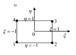
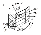
With finely layered bedding, the rock massif has the property of anisotropy [16]. The authors of this work have developed a model of an oblique-layered transtropic massif under conditions of generalized plane deformation. Figure 3 shows broad illustrations of the model in relation to studies of an anisotropic massif of a horizontally layered structure (Figure 3a), a drift (Figure 3b), a diagonal working (Figure 3c) and a crosscut (Figure 3d) located in the rock massif with an inclined structure lying at angles φ and ψ relative to the horizontal plane.
(a) Horizontally layered anisotropic massif
(b) Drift
(c) Diagonal working out
(d) Crosscut
Figure 3. Geometric illustrations of an anisotropic rock massif obliquely layered
Using the formula for the rotation of Lekhnitsky [14] coordinate systems, for the rotation of coordinate systems around the OY axis associated with the angle φ, for the elasticity coefficients dij (i=1, 2, ⋯, 6, j=1, 2, ⋯, b), Yerzhanov et al. [16] obtained the following expressions for the drift-shaped working:
$d_{11}=c_{11} \cos ^{4}(\varphi)+c_{33} \sin ^{4}(\varphi)+2\left(c_{13}+2 c_{44}\right) \sin ^{2}(\varphi) \cos ^{2}(\varphi)$
$d_{12}=c_{12} \cos ^{2}(\varphi)+c_{13} \sin ^{2}(\varphi)$
$d_{13}=c_{13}+\left(c_{11}+c_{33}-2 c_{13}-4 c_{44}\right) \sin ^{2}(\varphi) \cos ^{2}(\varphi)$
$d_{15}=\left(c_{11} \cos ^{2}(\phi)-\left(c_{13}+2 c_{44}\right)\right.$
$\left.\cos (2 \phi)-c_{33} \sin ^{2}(\phi)\right) \cos (\phi) \sin (\phi)$
$d_{22}=c_{11}$
$d_{23}=c_{12} \sin ^{2}(\varphi)+c_{13} \cos ^{2}(\varphi)$
$d_{25}=\left(c_{12}-c_{13}\right) \cos (\varphi) \sin (\varphi)$
$d_{33}=c_{11} \sin ^{4}(\phi)+c_{33} \cos ^{4}(\phi)$
$+2\left(c_{13}+2 c_{44}\right) \cos ^{2}(\phi) \sin ^{2}(\phi)$
$d_{35}=\left(c_{11} \sin ^{2}-c_{33} \cos ^{2}(\phi)\right.$
$\left.+\left(c_{13}+2 c_{44}\right) \cos (2 \phi)\right) \cos (\phi) \sin (\phi)$
$d_{44}=c_{44} \cos ^{2}(\varphi)+c_{66} \sin ^{2}(\varphi)$
$d_{46}=\left(c_{66}-c_{44}\right) \cos (\varphi) \sin (\varphi)$
$d_{55}=c_{44}+\left(c_{11}-2 c_{13}+c_{33}-4 c_{44}\right) \cos ^{2}(\varphi) \sin ^{2}(\varphi)$
$d_{66}=c_{44} \sin (\varphi) \cos (\varphi)+c_{66} \cos ^{2}(\varphi)$ (10)
In these expressions, 13 coefficients will be nonzero. Now, if we rotate the extended working axis coinciding with the OY axis in Figure 1b, by turning by the angle ψ around the OZ axis in the OX direction, they obtained the following 21 nonzero elastic coefficients for the crosscut and diagonal working, which are calculated by the expressions:
$d_{11}^{\prime}=d_{11} \cos ^{4}(\psi)+d_{22} \sin ^{4}(\psi)+2\left(d_{12}+\right.$
$\left.2 d_{66}\right) \cos ^{2}(\psi) \sin ^{2}(\psi)$,
$d_{12}^{\prime}=d_{12}+\left(d_{11}+d_{22}-4 d_{66}-\right.$
$\left.2 d_{12}\right) \cos ^{2}(\psi) \sin ^{2}(\psi)$,
$d_{13}^{\prime}=d_{13} \cos ^{2}(\psi)+d_{23} \sin ^{2}(\psi)$,
$d_{14}^{\prime}=\left(d_{15}-2 d_{46}\right) \cos ^{2}(\varphi) \sin (\psi)+$
$d_{25} \sin ^{3}(\psi)$,
$d_{15}^{\prime}=d_{15} \cos ^{2}(\psi)+\left(d_{25}+\right.$
$\left.2 d_{46}\right) \sin ^{2}(\psi) \cos (\psi)$,
$d_{16}^{\prime}=\left(d_{11}-2 d_{66}-d_{12}\right) \cos ^{3}(\psi) \sin (\psi)+$
$\left(d_{12}+2 d_{66}-d_{22}\right) \sin ^{3}(\psi) \cos (\psi)$,
$d_{35}^{\prime}=d_{35} \cos (\psi)$,
$d_{36}^{\prime}=\left(d_{13}-d_{23}\right) \sin (\psi) \cos (\psi)$,
$d_{44}^{\prime}=d_{44} \cos ^{2}(\psi)+d_{55} \sin ^{2}(\psi)$,
$d_{45}^{\prime}=\left(d_{55}-d_{44}\right) \sin (\psi) \cos (\psi)$,
$d_{46}^{\prime}=d_{46} \cos ^{3}(\psi)+\left(d_{15}-d_{46}-\right.$
$\left.d_{25}^{\prime}\right) \sin ^{2}(\psi) \cos (\psi)$,
$d_{55}^{\prime}=d_{44} \sin ^{2}(\psi)+d_{55} \cos ^{2}(\psi)$,
$d_{56}^{\prime}=d_{46} \cos ^{2}(\psi) \sin (\psi)+\left(d_{15}-d_{25}-\right.$
$\left.d_{46}\right) \cos ^{2}(\psi) \sin (\psi)$,
$d_{66}^{\prime}=d_{66}+\left(d_{11}+d_{22}-2 d_{12}-\right.$
$\left.4 d_{66}\right) \cos ^{2}(\psi) \sin (\psi)$ (11)
If we take ψ=0, then expressions (11) turn into expression (10), which describes the drift. If we take φ=0 in expressions (9), then we pass to the model of the anisotropic massif of a horizontally layered structure of Lekhnitsky [14]. If in expressions (7) and (9) we take E1=E2 and ν1=ν2, then we pass to the classical isotropic model, which is determined by two parameters of elasticity: E and ν.
In this article, it is proposed to easily apply the discussed model of the massif of an inclined-layered structure to a solid mass of soil of the landslide slope, which are formed by strata of inclined layers as a result of chemical weathering and denudation processes.
Now let’s write down the basic equation of the finite element method: a system of the equilibrium equations for the hillside soils of Ak Kain:
$[R]\{U\}=\left\{P^{d r y}\right\}+\left\{P^{\text {satur }}\right\}$ (12)
where, {Pdry} and {Psatur} are vectors of the volumetric forces from the action of the own gravitation weight of the soil for the H depth of the dry and water-saturated states. They are determined in layers by the volumetric weights of dry $\gamma_{n}^{d r y}$ and water-saturated $\gamma_{m}^{\text {satur }}$ soils from the rain infiltration. Here n and m are amounts of dry and water-saturated zones of the slope, m≪n.
The data for loamy soils of isotropic and anisotropic structure is available in ref. [18]. Using the described algorithm (1) - (12), the components of displacements, strains, and stresses are completely determined. Now one of the main issues remains selecting the criterion for determining the critical state of the soil before destruction.
The fracture mechanism for rocks is understood as the concept of the theory of elasticity: fault-upward, downward, reverse-upward, downward and transverse shear failure, and for soils of slopes, it means downward fault and separation failure. Upthrust and strike-slip destruction of soils on mountain slopes has not yet been observed. Thus, for soils the fracture mechanism is determined by the normal component of compressive stresses σn and separation failure, which is determined by the normal component of the tangential component of stresses +τn Here, the (+) sign means the direction of movement of the landslide soil mass down the slope from the observation point. These mechanisms after the destruction of the soil, that is, after the loss of stability, further movement will occur due to gravitational flattening.
Under the action of an external load at the internal points of the elastic massif, the effective forces can exceed the internal adhesion forces between the particles. In such cases, there begins the process of sliding of one particle over the other. If it is a soil massif, then the destruction of the soil begins, i.e. soil strength will be surpassed. It is known that in geometric terms the Coulomb–Mohr criteria is the equation of a straight line of the following form:
$\tau_{c}=C+\sigma_{n} \operatorname{tg} \varphi$ (13)
where, τc is a tangent component or displacement stress in the sliding area; C is the adhesion force; σn is the normal component of stresses in the sliding area; φ is the angle of internal friction. By successive steps (1)-(10), the stress components become known: σx, σz, τxz. Using them with the known relations of the theory of elasticity, the main stresses σmax, σmin, τmax and directions of the main areas are calculated: $\alpha=0.5 \operatorname{arctg} \frac{2 \tau_{x z}}{\sigma_{x-\sigma_{z}}}$. Critical tearing stresses σmax, σmin, τmax are taken from the laboratory data. Or, if critical values of the adhesion forces C and the angle of internal friction φ are known, the critical value of the tearing stresses τc is calculated by expression (13). Landslides on mountain slopes often occur by a mixed mechanism of normal pressure and shear stress.
The Calculation Model and Initial data of the Problem of Pre-Landslide State of the Ak Kain North-Western slope.
(a) The landslide pattern
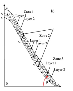
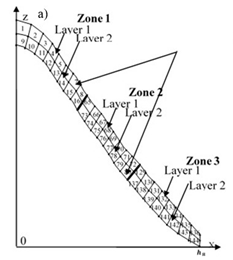
(b) Numbers of the calculated finite elements of two surface layers of the Ak Kain northern-west slope
Figure 4. Modeling the Ak Kain landslide
Figure 4a shows the cross section and the body of the Ak Kain landslide northern slope in 2004. The numbers show: 1 - landslide body; 2 – slopping line; 3- surface soil layer; 4 - exposed surface; 5 - final stop of the landslide mass movement 35 meters high; 6 - landslide front; 7 – pre-landslide surface of the hillside.
Figure 4b shows a fragment of the finite element model of the granite–basalt rock mountain together with surface soil layers (view from the North West to the South East side). For ease of analysis, the layers of the cover soil are divided into three zones. The thickness of the cover soil h layers is variable. The 1st layer thickness is: h1=2m, h2=7m, h3=12m, h4=1m. The 2nd layer thickness is: h5=5m, h6=9m, h7=11m, h8=1m. It also shows the layer numbers in the zones and the element numbers in them. The angle of slope θ=720.
The crucial moment of the proposed method, in addition to geometry, is preparation of the initial data on the PhM and strength properties. Such data for critical strategic facilities are established by drilling operations. Prior to the design stage of the Almaty Metro, such work was carried out. The territory of the city is located on the sloping foothill plain of the Zailiysky Mountains and directly adjoins the mountain slopes of the Northern Tien Shan. One high landslide hazardous mountain Kok Tobe is located in the territory of the city. The ridges of Zailiysky and Kungei Alatau of the Northern Tien Shan in the Miocene of the Tertiary period were raised to 2000 and 2500 meters (40 million years ago). In the Pliocene, these ridges had an almost modern shape (the last 25 million years ago). The formation of cover soils of this territory continues to nowadays, starting from the time of early Neotectonics due to sedimentation of cosmic dust, dedunation, chemical and other processes and weathering products.
Thus, the nature of the formation of predominantly loamy cover soils for the foothill slopes not only of Zailiysky Alatau but also for the entire system of mountain slopes of the Northern Tien Shan, such as Kok Tobe, Shym Bulak, Ak Bulak, Kol Sai and other is identical.
Reliable data on the PhMP of sand, sandy loam, loam, clay for these territories for soils of the isotropic and anisotropic structure for the foothill territory of the city of Almaty are available in work [19], the values of which are given in Tables 1 and 2.
The thicknesses of heterogeneous layers hk are different, they range from 2 meters to 6.5 meters. Their values are given in the last column of the Table. The total height of the columns, from which there were taken soil samples according to Table 1 is 41 m.
The novelty of this proposed approach is the developed mechanical-mathematical model for studying the landslide process, considering anisotropy of the soil structure in layers, since in nature cover soils of the slope rarely have a continuous homogeneous isotropic structure. Only loams have 8 varieties with different PhMP and strengths (1. Loam semi-solid. 2. Loam greenish-brown. 3. Loamy clay. 4. Loam brownish-brown. 5. Loam soft-plastic. 6. Loam plastic-elastic. 7. Loams of light brown color. 8. Loams of brown color) [20]. In fact, only the loamy structure of sloping soils is a heterogeneous environment, not to mention their mixtures with sandy loam, sand and clay. Tables 1-2 show some PhMP and strength properties of soils of anisotropic structure.
Since, according to the geological time, the foothill territory of the city of Almaty is a sloping plain and the mountain slopes listed above including Ak Kain, were formed simultaneously, at the first stage the FMS for various types of soils were taken from the data of Almatymetro, which are shown in Table 1.
The experimentally established values of FMS for soils with anisotropic structure are few. Some of such data are available in the work of Bugrov and Golubev [18]. Table 2 shows the values of FMS and strength properties for typical soils of mountain slopes are given in Table 2.
Table 1. Elastic properties of soils and their layers’ thicknesses on the path of the foothill territory of the city Almaty [10]
|
Layer k |
Soil |
Elastic constants |
Thickness hk, m |
|
|
Ek, MPa |
vk |
|||
|
1 2 3 4 5 6 7 8 9 10 |
Bulk Solid loam Loam with pebbles Gravel Boulder soil: with gravel; with pebbles Semi-solid loam Medium sand Pebbles with boulders Hard clay |
7.0 30.0 25.0 85.0 120.0 80.0 50.0 22.0 200.0 300.0 |
0.40 0.36 0.28 0.21 0.27 0.35 0.25 0.36 0.32 0.31 |
2.8 2.2 3.3 2.7 3.2 4.8 6.5 4.5 5.1 5.9 |
Table 2. PhMP and strength properties of anisotropic structure soils [12]
|
# |
Soils |
γ, kN/m3 |
E1, МPа |
E2, МPа |
G2, МPа |
ν1 |
ν2 |
C1, МPа |
C2, МPа |
$\varphi_{1}^{0}$ |
$\boldsymbol{\varphi}_{2}^{\mathbf{0}}$ |
|
1 |
Loam |
2.00 |
30.0 |
16.0 |
7.0 |
0.30 |
0.30 |
0.005 |
0.005 |
27 |
33 |
|
2 |
Priming |
1.90 |
10.00 |
15.0 |
7.6 |
0.36 |
0.24 |
0.030 |
0.060 |
19 |
23 |
|
3 |
Loam, wet |
0,94 |
6.0 |
4.0 |
1.7 |
0.39 |
0.35 |
0.050 |
0.007 |
15 |
18 |
|
4 |
Flowing sandy loam |
1.98 |
19.6 |
18.4 |
7.1 |
0.31 |
0.30 |
0.003 |
0.003 |
18 |
21 |
|
5 |
Fine sand |
2.11 |
81.3 |
85.0 |
32.7 |
0.28 |
0.30 |
0.002 |
0.002 |
35 |
37 |
|
6 |
Rock massif |
2.40 |
1074.0 |
523.0 |
0.12 |
0.41 |
0.20 |
39.00 |
21.00 |
21.0 |
12.0 |
Similar data for loamy and other types of anisotropic structure soils depending on the degree of humidity are available in work [20].
Figure 5 shows one of such graphical dependencies E0=E0(w). Here, the value of the deformation modulus E decreases nonlinearly with increasing the soil moisture.
There is the following relationship between the modulus of elasticity E and the modulus of deformation E0 [21]:
$E=E_{0}(1-2 v)$ (14)
where, ν is the Poisson coefficient.
Figure 5. Young module Е dependence on the soil humidity W [18]
The cross section of the slope in Figures 1 and 4a is divided into 384 elements with 425 nodal points along with the slope. To analyze the SSS of the surface layers of the slope where the landslide occurred, Figure 4 shows the numbers of zones and two layers of surface soil of the North-Western Ak Kain slope. So the number of zones 1 corresponds to the numbers 1-8 of the first layer and 9-16 of the second layer. Similarly, zone 2 corresponds to the element numbers: 62 - 72, 73 - 80 and the third zone to the numbers 129 - 136 and 137 - 144.
The results of FEM modeling using algorithms (1) - (12) of the studies and calculated values of stresses σx, σz, τxz. and σmax, σmin, τmax are given in Table 3. The numerator shows the research results for the option of dry slope soil and in the denominator for water-saturated soil with the moisture content of 41 %.
Table 3. Values of the stress components σx, σz, τxz and the main stresses in the elements of the first two layers of the surface soil of the Ak Kain slope
|
Ak Kain landslide northern slope |
||||||||||||
|
Zones No. |
Layers No. |
Elements No |
Stress components in elements, MPa |
ZonesNo. |
Layers No |
Elements No |
Critical stresses, MPa |
Critical areas, degree |
||||
|
σx |
σz |
τxz |
$\sigma_{\max }$ |
$\sigma_{\min }$ |
$\tau_{\max }$ |
σx |
||||||
|
I |
1 |
5 6 7 8 |
-0.10/-0.01 -0.13/-0.03 -0.14/-0.01 -0.21/0.00 |
-0.29/-0.05 -0.51/-0.07 -0.84/-0.06 -1.40/-0.05 |
0.12/0.00 0.22/0.00 0.31/0.01 0.60/0.00 |
I |
1 |
5 6 7 8 |
0.14/-0.11 0.24/-0.05 0.32/0.03 0.24/0.03 |
-0.23/-0.13 -0.42/-0,08 -0.73/-0.04
-1.27/-0.03 |
0.016/0.01 0.33/0.02 0.53/0.03 0.76/0.03 |
58/-39 61/72 62/82 64/87 |
|
2 |
13 14 15 16 |
-0.11/-0.02 -0.13/-0.02 -0.15/0.01 -0.27/0.02 |
-0.31/-0.09 -0.53/-0.10 -0.87/-0.08 -1.11/-0.08 |
0.13/-0.01 0.22/-0.01 0.33/-0.02 0.59/-0.03 |
2 |
13 14 15 16 |
0.14/-0.11 0.24/-0.03 0.30/0.05 0.27/0.04 |
-0.25/-0.17 -0.45/-0.10 -0.79/-0.06 -1.24/-0.06 |
0.20/0.05 0.34/0.03 0.55/0.04 0.76/0.06 |
59/-65 61/-83 63/-82 64/-79 |
||
|
II |
1 |
65 66 67 78 69 70 |
-0.65/-0.01 -0.63/-0.05 -0.61/-0.08 -0.49/-0.11 -0.30/-0.14 -0.97/-0.18 |
-1.15/-0.04 -0.79/-0.05 -0.56/-0.07 -0.32/-0.07 -0.14/-0.06 -0.05/-0.05 |
0.77/0.03 0.70/0.04 0.57/0.05 0.38/0.05 0.19/0.04 0.06/0.01 |
II |
1 |
65 66 67 68 69 70 |
-0.10/0.06 0.13/0.02 0.08/-0.05 0.06/-0.06 -0.00/-0.06 -0.03/-0.06 |
-1.75/-0.01 -1.33/-0.05 -1.11/-0.12 -0.77/-0.15 -0.42/-0.16 -0.13/-0.17 |
0.82/0.04 0.73/0.04 0.60/0.05 0.41/0.05 0.21/0.0 0.05/0.05 |
58/53 51/42 47/34 41/23 34/13 19/20 |
|
2 |
73 74 75 76 77 78 |
-0.59/0.02 -0.59/-0.01 -0.54/-0.06 -0.43/-0.09 -0.28/-0.13 -0.15/-0.17 |
-1.12/-0.09 -0.83/-0.11 -0.61/-0.14 -0.40/-0.14 -0.24/-0.14 -0.14/-0.12 |
0.72/0.02 0.66/0.04 0.54/0.05 0.38/0.06 0.22/0.04 0.11/0.02 |
2 |
73 74 75 76 77 78 |
-0.07/-0.22 0.10/-0.29 0.05/-0.28 -0.01/-0.23 -0.07/-0.03 -0.10/-0.02 |
-1.64/-0.40 -1.30/-0.41 -1.00/-0.41 -0.79/-0.48 -0.51/-0.48 -0.27/-0.25 |
0.78/0.07 0.70/0.05 0.57/0.05 0.39/0.05 0.22/0.05 0.08/0.05 |
58/71 52/59 49/49 46/36 42/22 39/29 |
||
The analysis of the values of stress components σx, σz, τxz according to Table 3 shows that at the boundaries of zones 1 and 2 where there is a junction where the lower boundary of eluvial deposits ends (Figure 6c), their value increases.
They correspond to the numbers of elements of the 1st layer 6, 7, 8, 65, 66, 67 and 68; local concentrations τxz and vertically downward compressing (pressing) σz stresses are observed. The same picture is observed at the foot of the slope in zone 3 in elements numbered 133, 134, 135 and 136, according to the separation stresses τxz and the shear stress σx. Their numerical values corresponding to these numbers are given in Table 3.
For clarity, Figures 6a, 6b, 6c, and 6d show their diagrams by zones and by layers. The revealed areas of stress concentration for the case of solid dry soil are shown in yellow, and for water-saturated layers in blue.
(a) Geological structure of the slope with FEM breakdown and stress diagrams at the centers of gravity of surface elements
(b) Diagram of the horizontal component σx
(c) Diagram of the tangent component τxz
(d) The vertical component of σz
Figure 6. Analysis of stress diagrams
The thicknesses of the layers of the four sections of the first layer in height in the vertical direction are equal to: h1=2m, h2=7m, h3=12m, h4=1m, of the second layer h5=2m, h6=7m, h7=12m, h8=1m. The total thickness of the two layers is: h12=7m, h22=16m, h32=23m, h42=2m. These tables correspond to the centers of gravity of the elements, and the corresponding numbers of zones, layers and elements are shown in Figure 6a. The inclination angle of the North-West slope "Ak Kain" θ=76°.
All three stress components are involved in the mechanism of separating a part of the soil mass on the slope: the beginning of the landslide process. Figure 6b shows the separation stress diagram τxz. The direction of this component is positive, with a plus sign and is directed from the surface of the slope at an angle downward, that is, it works for separation. Its greatest value is concentrated on the upper part of the slope and in the areas of the foot.
The horizontal stress component σx which diagram is shown in Figure 6с, is also tensile with the plus sign, is also directed to the right, the direction is shown by an arrow. But the greatest concentrated value is observed at the foot of the slope.
The diagram of the component σzthat is the main gravitational compressive stress is shown in Figure 6d with the minus sign. Their highest values are also localized in the slope region closer to the peak, in the first layer at the boundaries of zones I and II. Note that, as a result, the total effect of the stress components σx and σz at each point on the surface of the steep slope at the depths from 2 m to 4 m is directed to the right, down and approximately coincides with the direction of the shear stress τxz. The value of the total work of disruption, judging by the diagrams of stresses, corresponds to the vault area. These places are specifically shown in the right Figure 3 and in Figure 6a as zone 1. These places are precisely the area of the beginning of the landslide. As can be seen from the stress diagrams of Figure 6c, 6d, a strong stress concentration is observed here. And in Table 3, in elements 7 and 8 of the first layer and in elements 15 and 16 of the second layer, as well as at the transition to the second zone in the first layer in element 65, the highest values of compressive σz and disruption τxz stresses are observed. In the right Figure 1 these places are shown as the walls of the landslide disruption.
As the authors of works [4], rightly show in their studies, the landslide mass that started from the collapse wall simultaneously captures additional attached soil masses. Our research also found slope locations vulnerable to disruption. This second region has an increased stress concentration below in the area of the foot of the slope, the diagrams of which are shown in Figures 6b and 6с. With the Ak Kain landslide, the total mass of demolished soil was more than 1 million tons, and the remains are located at the foot (Figure 1a). Before the tragic landslide there, under the feet of one of our authors, at the depth of about 30 meters, there was a 2-storey residential building and farm buildings.
Now let us return to Figure 1. The remains of the landslide mass about 100 m long, 40 -50 m wide and about 30 m high (Figure 1a) are about 10 times larger than the volume of the mass of soil disrupted from the wall at the starting point (Figure 1b). This suggests that a huge ground mass was captured along the way. They correspond to places of a high stress concentration at the foot of the slope (Figures 6b and 6с).
The analysis of the main stresses is also important, the values of which are given in Table 3. If in the previous analysis we found the stress values at the centers of gravity of isoparametric elements, then here we can judge the stresses on the so-called main sites that lie at angles a. Judging by the data in Table 3, here also the main stresses σmax, σmin and τmax take their maximum values, as well as σx, σz, and τxz, at the boundary of zones 1, 2 and at the foot of the slope. The values of the principal stresses are slightly higher than the values of the stress components σx, σz, and τxz.
The angle a of the main sites relative to the horizontal axis 0X decreases almost smoothly from the value a=640 at the boundary of zones 1 and 2, reaching up to a=150. It is known from physics of the process that the steeper the center of gravity of masses above the floor, the more unstable it becomes. In this case, these are the masses of soils in the area of the arch of the slope, which have maximum disruption stresses that are vulnerable to disruption.
One of the numerical methods of studying the landslide process with the development of a method of mechanical-and-mathematical modeling of soils of the complex anisotropic structure hillside is proposed. Anisotropy of the soil lies in the natural structure of the soil, which consists not only of up to 8 types of loam varieties but also of the mixtures with sandy loams, clays, as well as an insignificant amount of sand.
For reliability of the methodology and model, one of the tragic landslides of the Northern Tien Shan ‘Ak Kain’ was reconstructed. The site, the geometry of the slope, the soil composition of the remains of the landslide mass and the path of its advancement were preliminarily examined. The PhMP and strength properties of the soils were mainly determined based on the data of drilling the foothill plain to the design stage of the Almaty Metro. Studying the remains of the soil, the geometry of its area and the angle of inclination of the slope showed that the two-layer structure of its original structure made a curved path repeating the outline of the gorge. Thus, the soil deposits of the slope together with the granite-basalt rock base are modeled by the finite element method as close as possible to the landslide initial shape. The key points of the mathematical model for solving the problem are briefly described.
The SSS of the North-Western slope of this mountain was determined for two variants of its condition: dry and water-saturated. The analyzes were performed on the stress components σx, σz, τxz, and the main stresses σmax, σmin, τmax, for the upper, middle and lower zones of the inclined slope and in its layers. There were established places with respect to the highest stress concentration. For all three stress components, the place of greatest concentration turned out to be where the disruption of the ground mass began. This place is zone 1, closer to the arch of the slope. A study using this technique showed that there was actually a stress concentration in the third zone, which belongs to the foot of the slope. Insignificant water saturation of the soil with the moisture content of 41% from spring rains will additionally increase the stress concentration. Such places for the dry state of the soil are shown by stress plots and elements in zones and layers are colored in yellow and places from water saturation are colored in blue. The geometry and volume of the remains indicate that the mass of landslide that disrupted from the wall (Figure 1) simultaneously captured the soil located in the same pre-landslide state in the third zone, closer to the area of the foot of the mountain slope.
Thus, the picture of the pre-landslide stress state of the cover soils of the Ak Kain hillside in dry and water-saturated conditions have been reconstructed.
In conclusion we note that the results of studies using the method of mathematical modeling allows stating its high reliability.
The proposed technique, method and model, taking into account anisotropy of the structure of slope soils, has been tested for reconstruction of the past landslide. This development makes it possible to predict the places of occurrence of possible dangerous pre-landslide conditions, not only of the numerous slopes of the Northern Tien Shan, the foothills of which are already densely populated but also of any landslide-prone mountain slopes, by determining dangerous stress concentrations.
[1] Chuvash Encyclopedia. http://enc.cap.ru/.
[2] Center for Expertise, Research and Testing in Construction. https://ceiis.mos.ru/.
[3] Deluvial slopes. https://helpiks.org/8-516.html
[4] Colluvium. https://ru.wikipedia.org/wiki/%D0%9A%D0%BE%D0%BB%D0%BB%D1%8E%D0%B2%D0%B8%D0%B9.
[5] Proluvium. https://ru.wikipedia.org/wiki/%D0%9F%D1%80%D0%BE%D0%BB%D1%8E%D0%B2%D0%B8%D0%B9.
[6] Longoni, L., Papini, M., Brambilla, D., Arosio, D., Zanzi, L. (2016). The role of the spatial scale and data accuracy on deep-seated gravitational slope deformation modeling: The Roncolandslide, Italy. Geomorphology, 253: 74-82. https://doi.org/10.1016/j.geomorph.2015.09.030
[7] Brunetti, M.T., Melillo, M., Peruccacci, S., Ciabatta, L., Brocca, L. (2018). How far are we from the use of satellite rainfall products inlandslide forecasting? Remote Sensing of Environment, 210: 65-75. https://doi.org/10.1016/j.rse.2018.03.016
[8] Kumar, M., Rana, S., Pant, P.D., Patel, R.C. (2017). Slope stability analysis of Balia Nala landslide, Kumaun Lesser Himalaya, Nainital, Uttarakhand, India. Journal of Rock Mechanics and Geotechnical Engineering, 9(1): 150-158. https://doi.org/10.1016/j.jrmge.2016.05.009
[9] Chen, K.T., Wu, J.H. (2018). Simulating the failure process of the Xinmo landslide using discontinuous deformation analysis. Engineering Geology, 239: 269-281. https://doi.org/10.1016/j.enggeo.2018.04.002
[10] Ran, Q., Hong, Y., Li, W., Gao, J. (2018). A modelling study of rainfall-induced shallow landslide mechanisms under different rainfall characteristics. Journal of Hydrology, 563: 790-801. https://doi.org/10.1016/j.jhydrol.2018.06.040
[11] Bulat, P.V., Zasukhin, O.N., Upyrev, V.V., Silnikov, M.V., Chernyshov, M.V. (2017). Base pressure oscillations and safety of load launching into orbit. Acta Astronautica, 135: 150-160. https://doi.org/10.1016/j.actaastro.2016.11.042
[12] Nordiana, M.M., Azwin, I.N., Nawawi, M.N.M., Khalil, A.E. (2018). Slope failures evaluation and lanslides investigation using 2-D resistivity method. NRIAG Journal of Astronomy and Geophysics, 7(1): 84-89. https://doi.org/10.1016/j.nrjag.2017.12.003
[13] Zenkevich, O. (1975). The finite element method in technology. Mir, Moscow.
[14] Lekhnitsky, S.G. (1965). The theory of elasticity of an anisotropic body. Gostekhizdat, Moscow.
[15] Yerzhanov, Z.S., Aitaliyev, S.M., Masanov, Z.K. (1971). Stability of horizontal workings in the inclined-layered massif. Nauka, Alma-Ata.
[16] Yerzhanov, Z.S., Aitaliyev, S.M., Massanov, Z.K. (1980). Seismic stress state of underground structures in a layered anisotropic massif. Nauka, Alma-Ata.
[17] Baimakhan, R.B. (2021). Development of a mechanical model of a rock mass of an obliquely layered structure for the design of engineering structures. In: Scientific Collection "InterConf" No. 48. Proceedings of the 8th International Scientific and Practical Conference "Challenges in Science of Nowadays" (April 4-5, 2021) at Washington, USA, 1005-1017.
[18] Bugrov, A.K., Golubev, A.I. (1993). Anisotropic soils and foundations of the structure. Nedra, St. Petersburg.
[19] Baimakhan, R.B. (2002). Calculation of the seismic stress state of underground structures in a heterogeneous strata by the finite element method. (Under the editorship of Sh.M. Aitaliev). Almaty.
[20] Dependence of the modulus of deformation of dusty clay soil on moisture. http://townevolution.ru/.
[21] Calculation of the modulus of elasticity of the soil | https://forum.dwg.ru./