Satyabrat Kar* | Nityananda Senapati | Bharat K. Swain | Minakshi Dash
© 2021 IIETA. This article is published by IIETA and is licensed under the CC BY 4.0 license (http://creativecommons.org/licenses/by/4.0/).
OPEN ACCESS
This paper study into the Magnetohydrodynamics (MHD) boundary layer flow with low pressure gradient over a horizontal plate in presence of viscous dissipation makes the study more interesting. A system of ordinary differential equations is formed from the nonlinear partial differential equations using suitable similarity transformation and then resolved by Homotopy perturbation method (HPM) as well as by Runge-Kutta mechanism with shooting Technique. Both numerical and analytical solutions are in good accountability with each other. The flow characteristics for different physical parameters are analysed through graphs and tables. All the calculations and figures are made using MATLAB. The important findings are: velocity of the fluid flow increases with increasing results of pressure gradient. At λ=0.05, it is almost linear and then gradually becomes curvy for higher values of pressure gradient, Greater values of Eckert number reduce the heat transfer. The broad execution of present study is demonstrated in polymer processing flows, cardio vascular system etc
boundary layer flow, HPM, MHD, pressure gradient, shooting technique, viscous dissipation
The concerned study about MHD boundary layer flow with viscous incompressible fluid flow has multitudinous applications in science; engineering era and industries such are textile industry, polymer technology, purification of crude oil, geothermal engineering, metal and polymer handling business, liquid metal and plasma flows and many more eras. Many Scientist and researchers have been received wide attention on this field. In view of these applications, Chen [1] has meticulously revealed the analytical solution of Magneto hydrodynamic flow of heat transfer with special types of viscoelastic fluids over a stretching sheet with energy dissipation, internal heat source and thermal emission. Moreover, huge attention has been drawn on fluid flow over a surface moving with either variable or constant velocity. Turkyilmazoglu [2] is the pioneer who reported the analytical solution of mixed convection with heat transmission of MHD viscoelastic fluid throughout a pervious stretching surface. Hayat et al. [3] have carried out their research on the three–dimensional fluid flow with generation/absorption of heat. The convective flow of micropolar fluid with isothermal porous surface moreover viscous dissipation and joule heating also well agreement by Rahman [4]. The MHD flow with unfreezing heat transmission of Cu-water nanofluid in connection with viscous dissipation and joule heating has observed by Hayat et al. [5]. Mahanthesh et al. [6] have introspected the effect of three-dimensional MHD flow of a nanofluid past a convectively heated stretching sheet with thermal emission and viscous dissipation. Khan et al. [7] focused the influence of the chemically reactive flow of micro polar fluid including viscous dissipation and Joule heating. Kumar [8] elucidated the influence of radiative heat conduction and viscous dissipation with hydro magnetic flow throughout a stretching surface in existence with heat flux. Sangapatnam et al. [9] have described the impact of emission and mass transfer on MHD flow past an impulsively isothermal perpendicular sheet with viscous dissipation. Kar et al. [10] have studied extensively the effect of chemical reaction and viscous dissipation on magneto hydrodynamic fluid flow including heat with mass transfer past a perpendicular porous plate.
The fluid flow throughout a horizontal plate plays a crucial role on both the theoretical and practical aspects because of inherent huge implementations in hydrometallurgical industries, chemical technology and plastic engineering. The wobbly MHD convective of nanofluids with boundary-layer flow over a extending sheet in addition with thermal emission and influence of viscous dissipation has analyzed by Khan et al. [11]. Motsumi and Makinde [12] have premeditated nanofluids flow throughout a pervious movable horizontal sheet due to showing of thermal radiation and viscous dissipation. This study has motivated by young researchers on fluid flow problems, which deals with a wide several boundary lawer problems with fluid flows over a stretching sheeting both Newtonian and non-Newtonian fluids. The study on MHD with the assorted convection heat transfer from rampant stretching sheet with due impact of viscous immoderation has been proposed by Partha et al. [13]. Vyas and Ranjan [14] have introspected on MHD flow with boundary conditions in a porous media over a stretching sheet in appearance of thermal emission with dissipation. Anjali and Ganga. [15] analysed the study on nonlinear MHD flow past a porous surface with irregularity of heat and dissipation effects. Ferdows et al. [16] have examined the boundary layer with MHD flow with heat transfer of a nanofluid throughout a permeable precarious stretching sheet with viscous dissipation. Nia et al [17] reported the effect of the steadiness of nonlinear differential equations by the strengthen of Homotopy Perturbation Technique. Venkateswarlu et al. [18] investigated the viscous dissipation effects on MHD flow over a movable surface along with constant heat source. Vajravelu et al [19] have investigated the volatile convective boundary layer viscous fluid flow with perpendicular surface and irregular fluid properties. Hunegnaw and Kishan [20] have premeditated the porous MHD heat and mass transfer flow throughout stretching sheet in porous media assuming with viscous dissipation and chemical reaction.
Although significant studies have been made on magnetic, radiative and electrically conducting flows from horizontal or vertical stretching sheets by researchers and sciencists. But the heat and mass diffusion along a perpendicular plate with viscosity of the natural convection flows has investigated by Dimian and Hadhoda [21].The natural convection of MHD of nanofluids with the impact of size, shape of nanoparticles and temperature of the base fluid studied by Reddy and Chamkha [22].The effects of chemical reaction and thermal emission in existence of viscosity of nanofluid flow throughout a permeable wedge ingrained in impregnated porous media inspected by James et al. [23]. The chemical reaction effects with heat and mass transfer through a porous medium of magnetohydrodynamics flow of nanofluids in existence with thermal emission, viscous dissipation experimented by Haile and Shankar [24]. An exponentially accelerated slanted plate immersed in a porous medium with thermal conductivity in existence of emission has inspected by Ahmmed et al. [25]. Hussain [26] is the pioneer who reported the solution for MHD nanofluid flow with heat and mass transfer across a porous surface with thermal emission, viscous dissipation as well as chemical reaction effect. Makinde and Mutuku [27] have evolved the MHD nanofluids with hydromagnetic thermal boundary layer flow throughout a heated horizontal plate with viscous dissipation and ohmic heating. The Lorentz force on convection nanofluid flow throughout a stretched sheet has meticulously scrutinized by Sheikholeslami et al. [28]. Kar et al. [29] have experimented the influence of the mass transfer effects on volatile convective MHD incompressible fluid flow along an exponentially accelerated perpendicular porous plate in the presence of heat source. Analytical solution of MHD flow along an imprudently commenced the perpendicular plate with the mass transfer effect also experimented by Swain and Senapati [30].
The preeminent purpose of the present paper is to quite develop the work of Jhankal [31] by considering heat transfer in presence of viscous dissipation. The irreversible process in which work done by the adjacent layer of fluid because of shearing forces is altered into heat is defined as viscous dissipation. It has many applications in real life world problem such are the aerodynamic heating in the thin boundary layer whereas the raises in the temperature of the skin of high speed aircraft. The reduced governing boundary layer equations are solved by Homotopy perturbation method and Runge-Kutta numerical integration with shooting technique. The comparison between the two methods proves the accuracy of solution.
Assume a two dimensional steady flow of a viscous incompressible fluid over a flat plate. Let us assume $T_{w}$ be the surface temperature of the sheet and the fluid of uniform ambient temperature $T_{\infty}$. All properties of fluid are speculated to constant. The $B_{0}$ is considered as transverse magnetic field, employed ordinarily to the plate while the produced magnetic field is imperceptible. Whereas it can be justified for MHD flow at insignificant magnetic Reynolds number and in energy equation Joule heating parameter is also spurned.
By employing boundary layer approximation, governing equations are as follow:
$\frac{\partial u}{\partial x}+\frac{\partial v}{\partial y}=0$ (1)
$u \frac{\partial u}{\partial x}+v \frac{\partial v}{\partial y}=-\frac{1}{\rho} \frac{\partial p}{\partial x}+v \frac{\partial^{2} u}{\partial y^{2}}-\frac{\sigma B_{0}^{2} u}{\rho}$ (2)
$u \frac{\partial T}{\partial x}+v \frac{\partial T}{\partial y}=\alpha \frac{\partial^{2} T}{\partial y^{2}}+\frac{v}{C_{P}}\left(\frac{\partial u}{\partial y}\right)^{2}$ (3)
Boundary conditions for the above problems are given by:
$\mathrm{u}(x, 0)=0, \mathrm{v}(x, 0)=0, \mathrm{~T}(x, 0)=T_{w}$
$\mathrm{u}(x, \infty) \rightarrow U_{\infty}, \mathrm{T}(x, \infty) \rightarrow T_{\infty}$ (4)
Introducing a stream function $\psi$ on Eq. (1) such as
$\mathrm{u}=\frac{\partial \psi}{\partial y}, \mathrm{v}=-\frac{\partial \psi}{\partial x}, \eta=y \sqrt{\frac{U_{\infty}}{v x}}, \psi=\sqrt{v x U_{\infty}} f(\eta),$$\theta(\eta)=\frac{T-T_{\infty}}{T_{w}-T_{\infty}}$ (5)
Using the above transformations into Eqns. (2) and (3).
Nonlinear transformed ordinary differential equations with $\eta$ as independent similarity variable are
$f^{\prime \prime \prime}+\frac{1}{2} f f^{\prime \prime}-M^{2} f^{\prime}=-\lambda$ (6)
$\theta^{\prime \prime}+\frac{P r}{2} \theta^{\prime} f+\operatorname{PrEcf}^{\prime \prime 2}=0$ (7)
And the reformed boundary conditions are
$f(0)=0, f^{\prime}(0)=0, \theta(0)=1, f^{\prime}(\infty) \rightarrow 1,$$\theta(\infty) \rightarrow 0$ (8)
where, prime denotes differentiation with regard to $\eta$, the pressure gradient is $\lambda=-\frac{x}{\rho U_{\infty}} \frac{d p}{d x}$, the dimensionless magnetic parameter is $M^{2}=\frac{\sigma B_{0}^{2}}{\rho} \frac{x}{U_{\infty}}$, the prandtl number is $P r=\frac{v}{\alpha}$ and the Eckert number is $\mathrm{Ec}=\frac{U_{\infty}^{2}}{C p\left(T_{w}-T_{\infty}\right)}$.
3.1 Homotopy perturbation method
Basic concept of homotopy perturbation method (HPM), we consider the following nonlinear differential equation:
$A(u)-f(r)=0, r \in \Omega$ (9)
Subject to the boundary conditions
$B\left(u, \frac{\partial u}{\partial \eta}\right)=0, r \in \Gamma$ (10)
where, $\mathrm{A}$ is a general differential operator, $\mathrm{B}$ is a boundary operator, $f(r)$ is a known an analytical function and $\Gamma$ is the boundary of the domain $\Omega$.
Operator A can be divided into two parts, which are L and N, where L is linear and N is nonlinear, therefore Eq. (9) can be
$L(u)+N(u)-f(r)=0 . r \in \Omega$ (11)
By the homotopy perturbation technique,
We construct a homotopy $U(r, p): \Omega \times[0,1] \rightarrow R$, which satisfies:
$\mathrm{H}(\mathrm{U}, \mathrm{p})=(1-p)\left[L(U)-L\left(u_{0}\right)\right]+p[A(U)-f(r)]$,$p \in[0,1] r \in \Omega$ (12)
where, $p \in[0,1]$ is an embedding parameter, $u_{0}$ is an initial approximation, which satisfies the boundary condition. Obviously, from these definitions we have
$\mathrm{H}(\mathrm{U}, 0)=\mathrm{L}(\mathrm{U})-L\left(u_{0}\right)=0$, $\mathrm{H}(\mathrm{U}, 1)=\mathrm{A}(\mathrm{U})-f(r)=0$
The changing process of $p$ from zero to unity is just that of $U(r, p)$ from $u_{0}(r)$ to $u(r)$. In topology, $\mathrm{L}(\mathrm{U})-L\left(u_{0}\right)$ and $\mathrm{A}(\mathrm{U})-f(r)$ are called homotopy. According to the (HPM), we can first use the embedding parameter $p$ as a small parameter and assume that the solution of Eq. (12) can be written as a power series in $p$ :
$U=U_{0}+p U_{1}+p^{2} U_{2}+p^{3} U_{3}+\cdots$ (13)
Setting $p=1$, results in the approximate solution of Eq. (9)
$u=\lim _{p \rightarrow 1} U=U_{0}+U_{1}+U_{2}+U_{3}+\cdots$ (14)
Using Homotopy perturbation method, the homotopy forms of Eqns. (6) and (7) are given below:
$(1-p)\left(f^{\prime \prime \prime}-M^{2} f^{\prime}\right)+p\left(f^{\prime \prime \prime}+\frac{1}{2} f f^{\prime \prime}-M^{2} f^{\prime}\right)$$=-\lambda$ (15)
$(1-p)\left(\theta^{\prime \prime}\right)+p\left(\theta^{\prime \prime}+\frac{P r}{2} \theta^{\prime} f+\operatorname{PrEc} f^{\prime \prime^{2}}\right)=0$ (16)
Here we assume $f$ and $\theta$ as the following forms: -
$f=f_{0}+p f_{1}+p^{2} f_{2}+p^{3} f_{3}+p^{4} f_{4}$. $\cdots \ldots \ldots \ldots . .$
$\theta=\theta_{0}+p \theta_{1}+p^{2} \theta_{2}+p^{3} \theta_{3}+p^{4} \theta_{4} \ldots \ldots \ldots . .$ (17)
Substituting Eq. (17) into Eq. (15) and Eq. (16), we obtain independent term of $p$ as follow
$f_{0}^{\prime \prime \prime}-M^{2} f_{0}^{\prime}=-\lambda$ (18)
$\theta_{0}^{\prime \prime}=0$ (19)
The boundary conditions are
$f_{0}(0)=0, f_{0}^{\prime}(0)=0, f_{0}^{\prime}(\infty)=1, \theta_{0}(0)=1$, $\theta_{0}(\infty)=0 .$ (20)
Terms containing only $p$ are given below:
$f_{1}^{\prime \prime \prime}-M^{2} f_{1}^{\prime}+\frac{1}{2} f_{0}^{\prime \prime} f_{0}=0$ (21)
$\theta_{1}^{\prime \prime}+\frac{\operatorname{Pr}}{2} \theta_{0}^{\prime} f_{0}+\operatorname{PrEc} f_{0}^{\prime \prime^{2}}=0$ (22)
The boundary conditions are given below:
$f_{1}(0)=0, f_{1}^{\prime}(0)=0, f_{1}^{\prime}(\infty)=0, \theta_{1}(0)=0$, $\theta_{1}(\infty)=0$ (23)
Now, solving Eq. (18)-(19) and Eq. (21)-(22) with boundary conditions (20) and (23) respectively, we obtain
$f_{0}=C_{1}+C_{2} e^{M \eta}+C_{3} e^{-M \eta}+\frac{\lambda \eta}{M^{2}}$ (24)
$\begin{aligned} f_{1}=C_{4}+C_{5} e^{M \eta} &+C_{6} e^{-M \eta}+J_{3} \eta e^{M \eta}+J_{4} \eta e^{-M \eta} \\ &+J_{5} \eta^{2} e^{M \eta}+J_{6} \eta^{2} e^{-M \eta}+J_{7} e^{2 M \eta} \\ &+J_{8} e^{-2 M \eta}+J_{9} \end{aligned}$ (25)
$\theta_{0}=-\frac{\eta}{6}+1$ (26)
$\theta_{1}=C_{9}+C_{10} \eta+J_{11} e^{M \eta}+J_{12} e^{-M \eta}+J_{13} e^{2 M \eta}$$+J_{14} e^{-2 M \eta}+J_{15} \eta^{2}+J_{16} \eta^{3}$ (27)
The above assigned constant coefficients can be estimated using boundary conditions. η∞ is assumed as 6.
3.2 Numerical integration by Runge-Kutta technique
With due implementation of numerical integration, a set of first order differential equations is developed from Eqns. (6) and (7). We generate the following substitutions
$f=y_{1}, f^{\prime}=y_{2}, f^{\prime \prime}=y_{3}, \theta=y_{4}, \theta^{\prime}=y_{5}$ (28)
The reduced equations are
$\begin{aligned} y_{3}^{\prime} &=-\frac{1}{2} y_{1} y_{3}+M^{2} y_{2}-\lambda \\ y_{5}^{\prime} &=-\frac{P_{r}}{2} y_{1} y_{5}+P_{r} E_{c} y_{3}{ }^{2} \end{aligned}$ (29)
Corresponding boundary conditions are given by
$y_{1}=0, y_{2}=0, y_{3}=?, y_{4}=1, y_{5}=?$, at $\eta=0$ (30)
$y_{2} \rightarrow 1, y_{4} \rightarrow 0$ at $\eta \rightarrow \infty$. (31)
To initiate the integration, the result of y3 and y5 at η=0 are provided as guess values whereas the stepwise integration is employed with step interval 0.001 adopting shooting mechanism with code of MATLAB along with error bound 10-3.
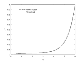
Here MHD flow of incompressible fluid over flat sheet has been analyzed in the existence of low pressure gradient and viscous dissipation. Suitable similarity transformation was used to acquire a system of ordinary differential equation from the employed nonlinear partial differential equations. The reduced system has been solved analytically by HPM and numerically by Runge-Kutta mechanism along with shooting technique. To validate our result, we compared the analytical solution [31] with the numerical solution taking M=1.5, λ=0.05 in Figure 9 and found a good agreement. Some other results are given below.
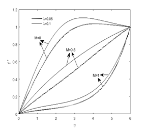
Figure 1. Velocity profile for λ when Pr=1, Ec=0.02, M=1
Figure 2. Velocity profile for M when Pr=1, Ec=0.02
Figure 1 and Figure 2 represents the velocity distribution for distinct values of pressure gradient and magnetic parameter M. It is noticed that the velocity of fluid flow increases with higher values of pressure gradient. At λ=0.05, it is almost linear and then gradually becomes curvy for surpassing values of pressure gradient. It has been shown that improve in magnetic field parameter M diminishes the velocity. The same result is also noticed in previous study by Jhankal [31]. The increasing values of M create a resistive force such as drag force which is called Lorentz force. The force on the velocity is retarded by Lorentz force and so motion gets slow down. Further it is clear that keeping magnetic parameter steady, velocity can be increased by increasing pressure gradient. That means the pressure gradient force take the fluid from high pressure zone to low pressure zone. This flow velocity and pressure gradient relation is clinically used to appraise coronary stenoses.
Figure 3. Temperature profile for Ec when λ =0.1, Pr=1, M=1
When temperature distribution is depicted for various Eckert number Ec=0, 0.1, 0.2, 0.3, it is found that temperature rises for higher values of Eckert number (Figure 3). Eckert number is defined as the ratio of kinetic energy flow and heat enthalpy difference whereas temperature is assumed as average kinetic energy. So here it can be mentioned that higher viscous dissipative heat raises the temperature significantly. This type of significant temperature rising is shown in polymer refining flows like injection moulding or extrusion at inflated rates.
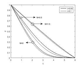
Figure 4. Temperature profile for λ when Pr=1, M=1
Figure 4 here temperature profiles are drawn for pressure gradient parameter λ=0, 0.05, 0.1 and 0.2. It is perceived that magnifying results of λ reduces the thermal boundary layer stratum.It is also perceived that pressure gradient parameter is inversely proportional to the temperature. Again for a fixed value of pressure gradient, higher Eckert number favours the temperature to improve as in Figure 3.
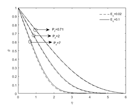
Figure 5 and Figure 6 illustrate that higher value of Prandtl number Pr results a diminishes in temperature. That means enhance in Prandtl number reduces the stratum of thermal boundary layer. Again Prandtl number is to diminish the temperature in the presence of higher pressure gradient whereas Pr makes the flow domain more hot with help of larger Eckert number.
Figure 5. Temperature profile for Pr when M=1, Ec=0.02
Figure 6. Temperature profile for Pr when λ=0.1, M=1
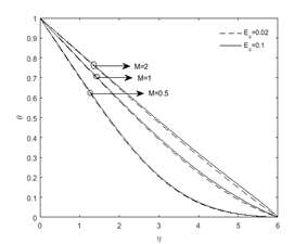
Variation in the temperature distribution is shown in Figure 7 and Figure 8 for several values of magnetic parameter M. With improve in M; there is a rise in temperature. Because higher magnetic parameter involves stronger Lorentz force which leads to a higher temperature. Further, if we see it is found that for a particular value of M, the outcomes of pressure gradient parameter and Eckert number on temperature are different i.e. just opposite.
Figure 7. Temperature profile for M when Pr=1, Ec=0.02
Figure 8. Temperature profile for M when Pr=1, λ=0.1
Figure 9. Comparison between HPM and RK method solution at M=1.5, λ=0.05
Table 1 presents the skin friction for dissimilar outcomes of magnetic parameter M and pressure gradient parameter λ. Higher values of M decreases the shearing stress whereas more pressure gradient enhances it.
Table 1. Numerical results of skin friction
|
SL.NO. |
M |
λ |
$f^{\prime \prime}(0)$ |
|
1 |
0.5 |
0.1 |
0.2960 |
|
2 |
1 |
0.1 |
0.1073 |
|
3 |
1.5 |
0.1 |
0.0671 |
|
4 |
0.5 |
0.05 |
0.1921 |
|
5 |
0.5 |
0.2 |
0.4949 |
Table 2. Numerical results of Nusselt number
|
SL.NO. |
M |
λ |
Pr |
Ec |
$-\theta^{\prime}(0)$ |
|
1 |
0.5 |
0.1 |
1 |
0.02 |
0.3009 |
|
2 |
1 |
0.1 |
1 |
0.02 |
0.2111 |
|
3 |
1.5 |
0.1 |
1 |
0.02 |
0.1862 |
|
4 |
0.5 |
0.05 |
1 |
0.02 |
0.2714 |
|
5 |
0.5 |
0.2 |
1 |
0.02 |
0.3466 |
|
6 |
0.5 |
0.1 |
0.71 |
0.02 |
0.2691 |
|
7 |
0.5 |
0.1 |
7 |
0.02 |
0.5861 |
|
8 |
0.5 |
0.1 |
1 |
0.1 |
0.2925 |
|
9 |
0.5 |
0.1 |
1 |
0.2 |
0.2820 |
Table 2 gives the numeric results of Nusselt number for the parameters M, Pr, λ and Ec. It is noted that larger values of pressure gradient and Prandtl number improves the rate of heat transfer. Contrarily magnetic parameter and Eckert number adversely affect the Nusselt number. Physically, if Eckert number is increased, temperature difference decreases and consequently the rate of heat transfer also gets slow down.
The authors are thankful to prof. Giulio Lorenzini, Editor-in-Chief, MMEP and the reviewers for their kind suggestion and comments for improvement of the manuscript.
|
E |
Electric field, kgm-1s-3 A-1 |
|||
|
Cp |
Specific heat at constant pressure, Jkg-1K |
|||
|
Ec |
Eckert number |
|||
|
Q |
Heat source parameter |
|||
|
Pr |
Prandtl number |
|||
|
T |
Dimensionless temperature, K |
|||
|
$T_{\infty}$ |
Temperature of the fluid in the free sream, K |
|||
|
u |
Velocity of x-component, ms-1 |
|||
|
v |
Velocity of y-component, ms-1 |
|||
|
P |
Pressure, kgm-1s-2 |
|||
|
$B_{0}$ |
Applied magnetic field |
|||
|
M |
Magnetic field parameter |
|||
|
Nu |
Nusselt number |
|||
|
t |
Dimensionless time |
|||
|
$T_{w}$ |
Fluid temperature at the plate, K |
|||
|
f |
Dimensionless free stream function |
|||
|
$U_{\infty}$ |
Free stream velocity, ms-1 |
|||
|
y |
Coordinate axis normal to the plate |
|||
|
Greek symbols |
||||
|
$\alpha$ |
Coefficient of thermal diffusivity |
|||
|
$v$ |
Kinematic viscosity, m2s-1 |
|||
|
$\lambda$ |
Pressure gradient parameter |
|||
|
$\sigma$ |
Electrical Conductivity, kg-1m-3s3A2 |
|||
|
$\psi$ |
Stream function |
|||
|
$\gamma$ |
Suction parameter |
|||
|
$\rho$ |
Density of fluid, kgm-3 |
|||
|
$\theta$ |
Dimensionless temperature, K |
|||
|
$\eta$ |
Dimensionless similarity variable |
|||
|
Subscripts |
||||
|
' |
derivative with regard to $\eta$ |
|||
|
w |
properties at the plate |
|||
|
$\infty$ |
free stream condition |
|||
$J_{1}=e^{M \eta}-e^{-M \eta}$
$J_{2}=\frac{\lambda}{M^{2}}\left(1-e^{-M \eta}\right) \quad C_{1}=-\left(C_{2}+C_{3}\right)$
$J_{3}=\left(-\frac{C_{1} C_{2}}{4}+\frac{3 \lambda C_{2}}{8 M^{3}}\right) \quad C_{2}=\frac{\left(1-J_{2}\right)}{M J_{1}}$
$J_{4}=\left(-\frac{C_{1} C_{3}}{4}-\frac{3 \lambda C_{3}}{8 M^{3}}\right) \quad C_{3}=\frac{\left(1-J_{2}\right)}{M J_{1}}+\frac{\lambda}{M^{3}}$
$J_{5}=-\frac{\lambda C_{2}}{8 M^{2}} \quad C_{4}=-\left(C_{5}+C_{6}+C_{7}+C_{8}\right)$
$J_{6}=-\frac{\lambda C_{3}}{8 M^{2}} \quad C_{5}=\frac{\left(J_{3}+J_{4}+2 M J_{7}-2 M J_{8}+J_{9}\right) e^{-M \eta}}{M J_{1}}-\frac{J_{10}}{M J_{1}}$
$J_{7}=-\frac{C_{2}^{2}}{12 M}$ $C_{6}=\left(C_{5}+2 J_{7}-2 J_{8}\right)+\frac{1}{M}\left(J_{3}+J_{4}+J_{9}\right)$
$J_{8}=\frac{C_{3}^{2}}{12 M}$ $C_{7}=1, \quad C_{8}=-\frac{1}{6}$
$J_{9}=C_{2} C_{3}$ $C_{9}=-\left(J_{11}+J_{12}+J_{13}+J_{14}\right)$
$J_{10}=\left(J_{3}+6 M J_{3}+12 J_{5}+36 M J_{5}\right) e^{M \eta}+\left(J_{4}-6 M J_{4}+12 J_{6}-36 M J_{6}\right) e^{-M \eta}+2 M J_{7} e^{2 M \eta}-2 M J_{8} e^{-2 M \eta}+J_{9}$
$J_{11}=\frac{\operatorname{Pr} C_{2}}{12 M^{2}}, J_{12}=\frac{\operatorname{Pr} C_{3}}{12 M^{2}}, J_{13}=-\frac{\operatorname{PrEcC}_{2}^{2} M^{2}}{4}, J_{14}=-\frac{\operatorname{PrEcC}_{3}^{2} M^{2}}{4}$
$J_{15}=\left(\frac{\operatorname{Pr} C_{1}}{24}-\operatorname{PrEcM}^{4} C_{2} C_{3}\right), J_{16}=\frac{\operatorname{Pr} \lambda}{72 M^{2}}$
$C_{10}=\frac{1}{6}\left(J_{11}+J_{12}+J_{13}+J_{14}-36 J_{15}-216 J_{16}\right)-$$\frac{1}{6}\left(J_{11} e^{6 M}+J_{12} e^{-6 M}+J_{13} e^{12 M} J_{14} e^{-12 M}\right)$
[1] Chen, C.H. (2010). On the analytic solution of MHD flow and heat transfer for two types of viscoelastic fluid over a stretching sheet with energy dissipation, internal heat source and thermal radiation. International Journal of Heat and Mass Transfer, 53(19-20): 4264-4273. https://doi.org/10.1016/j.ijheatmasstransfer.2010.05.053
[2] Turkyilmazoglu, M. (2013). The analytical solution of mixed convection heat transfer and fluid flow of a MHD viscoelastic fluid over a permeable stretching surface. International Journal of Mechanical Sciences, 77: 263-268. https://doi.org/10.1016/j.ijmecsci.2013.10.011
[3] Hayat, T., Shehzad, S.A., Qasim, M., Asghar, S. (2014). Three-dimensional stretched flow via convective boundary condition and heat generation/absorption. International Journal of Numerical Methods for Heat & Fluid Flow, 24(2): 342-358. https://doi.org/10.1108/HFF-03-2012-0065
[4] Rahman, M.M. (2009). Convective flows of micropolar fluids from radiate isothermal porous surfaces with viscous dissipation and Joule heating. Communications in Nonlinear Science and Numerical Simulation, 14(7): 3018-3030. https://doi.org/10.1016/j.cnsns.2008.11.010
[5] Hayat, T., Imtiaz, M., Alsaedi, A. (2016). Melting heat transfer in the MHD flow of Cu–water nanofluid with viscous dissipation and Joule heating. Advanced Powder Technology, 27(4): 1301-1308. https://doi.org/10.1016/j.apt.2016.04.024
[6] Mahanthesh, B., Gireesha, B.J., Gorla, R.S.R. (2017). Unsteady three-dimensional MHD flow of a nano Eyring-Powell fluid past a convectively heated stretching sheet in the presence of thermal radiation, viscous dissipation and Joule heating. Journal of the Association of Arab Universities for Basic and Applied Sciences, 23: 75-84. https://doi.org/10.1016/j.jaubas.2016.05.004
[7] Khan, M.I., Waqas, M., Hayat, T., Alsaedi, A. (2017). Chemically reactive flow of micropolar fluid accounting viscous dissipation and Joule heating. Results in Physics, 7: 3706-3715. https://doi.org/10.1016/j.rinp.2017.09.016
[8] Kumar, H. (2009). Radiative heat transfer with hydromagnetic flow and viscous dissipation over a stretching surface in the presence of variable heat flux. Thermal Science, 13(2): 163-169. https://doi.org/10.2298/TSCI0902163K
[9] Sangapatnam, S., Nandanoor, R.B., Vallampati, P.R. (2009). Radiation and mass transfer effects on MHD free convection flow past an impulsively started isothermal vertical plate with dissipation. Thermal Science, 13(2): 171-181. https://doi.org/10.2298/TSCI0902171S
[10] Kar, S., Senapati, N., Swain, B.K. (2019). Effect of chemical reaction on MHD flow with heat and mass transfer past a vertical porous plate in the presence of viscous dissipation. Bulletin of Pure and Applied Sciences, 38(1): 450-465. https://doi.org/10.5958/2320-3226.2019.00049.3
[11] Khan, M.S., Karim, I., Ali, L.E., Islam, A. (2012). Unsteady MHD free convection boundary-layer flow of a nanofluid along a stretching sheet with thermal radiation and viscous dissipation effects. International Nano Letters, 2(1): 1-9. https://doi.org/10.1186/2228-5326-2-24
[12] Motsumi, T.G., Makinde, O.D. (2012). Effects of thermal radiation and viscous dissipation on boundary layer flow of nanofluids over a permeable moving flat plate. Physica Scripta, 86(4): 045003. https://doi.org/10.1088/0031-8949/86/04/045003
[13] Partha, M.K., Murthy, P.V.S.N., Rajasekhar, G.P. (2005). Effect of viscous dissipation on the mixed convection heat transfer from an exponentially stretching surface. Heat and Mass Transfer, 41(4): 360-366. https://doi.org/10.1007/s00231-004-0552-2
[14] Vyas, P., Ranjan, A. (2010). Dissipative MHD boundary-layer flow in a porous medium over a sheet stretching nonlinearly in the presence of radiation. Applied Mathematical Sciences, 4(61-64): 3133-3142.
[15] Anjali, D.S., Ganga, B. (2010). Dissipation effects on MHD nonlinear flow and heat transfer past a porous surface with prescribed heat flux. Journal of Applied Fluid Mechanics, 3(1): 1-6.
[16] Ferdows, M., Chapal, S.M., Afify, A.A. (2014). Boundary layer flow and heat transfer of a nanofluid over a permeable unsteady stretching sheet with viscous dissipation. Journal of Engineering Thermophysics, 23(3): 216-228. https://doi.org/10.1134/S1810232814030059
[17] Nia, S.H., Ranjbar, A.N., Ganji, D.D., Soltani, H., Ghasemi, J. (2008). Maintaining the stability of nonlinear differential equations by the enhancement of HPM. Physics Letters A, 372(16): 2855-2861. https://doi.org/10.1016/j.physleta.2007.12.054
[18] Venkateswarlu, B., Narayana, P.S., Tarakaramu, N. (2018). Melting and viscous dissipation effects on MHD flow over a moving surface with constant heat source. Transactions of A. Razmadze Mathematical Institute, 172(3): 619-630. https://doi.org/10.1016/j.trmi.2018.03.007
[19] Vajravelu, K., Prasad, K.V., Ng, C.O. (2013). Unsteady convective boundary layer flow of a viscous fluid at a vertical surface with variable fluid properties. Nonlinear Analysis: Real World Applications, 14(1): 455-464. https://doi.org/10.1016/j.nonrwa.2012.07.008
[20] Hunegnaw, D., Kishan, N. (2014). Unsteady MHD heat and mass transfer flow over stretching sheet in porous medium with variable properties considering viscous dissipation and chemical reaction. American Chemical Science Journal, 4(6): 901-917.
[21] Dimian, M.F., Hadhoda, M.K. (2004). Natural convection flows with variable viscosity, heat and mass diffusion along a vertical plate. Mechanics and Mechanical Engineering, 7(2): 61-76.
[22] Reddy, P.S., Chamkha, A.J. (2016). Influence of size, shape, type of nanoparticles, type and temperature of the base fluid on natural convection MHD of nanofluids. Alexandria Engineering Journal, 55(1): 331-341. https://doi.org/10.1016/j.aej.2016.01.027
[23] James, M., Mureithi, E.W., Kuznetsov, D. (2015). Effects of variable viscosity of nanofluid flow over a permeable wedge embedded in saturated porous medium with chemical reaction and thermal radiation. International Journal of Advances in Applied Mathematics and Mechanics, 2(3): 101-118.
[24] Haile, E., Shankar, B. (2014). Heat and mass transfer through a porous media of MHD flow of nanofluids with thermal radiation, viscous dissipation and chemical reaction effects. American Chemical Science Journal, 4(6): 828-846.
[25] Ahmmed, S.F., Biswas, R., Afikuzzaman, M. (2018). Unsteady magnetohydrodynamic free convection flow of nanofluid through an exponentially accelerated inclined plate embedded in a porous medium with variable thermal conductivity in the presence of radiation. Journal of Nanofluids, 7(5): 891-901. https://doi.org/10.1166/jon.2018.1520
[26] Hussain, S. (2017). Finite element solution for MHD flow of nanofluids with heat and mass transfer through a porous media with thermal radiation, viscous dissipation and chemical reaction effects. Advances in Applied Mathematics and Mechanics, 9(4): 904-923. https://doi.org/10.4208/aamm.2014.m793
[27] Makinde, O.D., Mutuku, W.N. (2014). Hydromagnetic thermal boundary layer of nanofluids over a convectively heated flat plate with viscous dissipation and ohmic heating. UPB Sci Bull Ser A, 76(2): 181-192.
[28] Sheikholeslami, M., Mustafa, M.T., Ganji, D.D. (2016). Effect of Lorentz forces on forced-convection nanofluid flow over a stretched surface. Particuology, 26: 108-113. https://doi.org/10.1016/j.partic.2016.01.001
[29] Kar, S., Senapati, N., Swain, B.K. (2020). Mass transfer effect on unsteady convective MHD flow of incompressible fluid past an exponentially accelerated vertical porous plate in the presence of heat source, International Journal of Mathematics and Computation, 31(1): 54-66.
[30] Swain, B.K., Senapati, N. (2015). The effect of mass transfer on mhd free convective radiating flow over an impulsively started vertical plate embedded in a porous medium. Journal of Applied Analysis & Computation, 5(1): 18-27.
[31] Jhankal, A.K. (2014). Homotopy perturbation method for MHD boundary layer flow with low pressure gradient over a flat plate. Journal of Applied Fluid Mechanics, 7(1): 177-185.