Younes Talaei | Hasan Hosseinzadeh* | Samad Noeiaghdam
© 2021 IIETA. This article is published by IIETA and is licensed under the CC BY 4.0 license (http://creativecommons.org/licenses/by/4.0/).
OPEN ACCESS
In this paper, we present a novel technique based on backward-difference method and Galerkin spectral method for solving Black–Scholes equation. The main propose of this method is to reduce the solution of this problem to the solution of a system of algebraic equations. The convergence order of the proposed method is investigated. Also, we provide numerical experiment to show the validity of proposed method.
Black–Scholes equation, generalized Jacobi polynomials, backward-difference method, numerical solution
The pricing of options is a main problem in financial investment. Because of both theoretical and practical importance then using options thrive in the financial market. In option pricing theory, the Black-Scholes equation is one of the most effective models for pricing options. Black-Scholes option pricing model (also called Black-Scholes-Merton Model) values a European-style call or put option based on the current price of the underlying (asset), the option’s exercise price, the underlying’s volatility, the option’s time to expiration and the annual risk-free rate of return [1]. Consider the Black-Scholes equation based on the following options:
$P_{t}(S, t)+\frac{1}{2} \sigma^{2} S^{2} P_{S S}(S, t)+r S P_{S}(S, t)-r P(S, t)$=0, (1)
with the conditions:
$P(S, T)=\max (E-S, 0), \quad S \in \Omega=[0, \infty)$
$P(0, t)=E e^{-r(T-t)}, \quad P(S, t)=0, \quad$ as $\quad S \rightarrow \infty$
where, $P(S, t)$ is the European call option price at asset price S and at time t, E is the exercise price, T is the maturity, r is the risk free interest rate, and $\sigma$ represents the volatility function of underlying asset. During the past few decades, many researchers studied the existence of solutions of the Black-Scholes model using many methods in papers [2, 3]. In general, closed-form analytical solutions of some of these Black-Scholes PDEs do not exist and therefore one has to resort to numerical methods in order to solve them. There is an enriched literature regarding the numerical solution of Black-Scholes PDE in finance using different strategies such as Ref. [4-8] and the references cited.
The spectral method plays a significant role in various fields of applied science, especially in fluid dynamics where a large spectral hydrodynamics codes are now regularly used to study turbulence, transition, numerical weather prediction, and ocean dynamics [9]. This method is built on approximating the series solutions for differential equations in terms of classical orthogonal polynomials (Legendre, Chebyshev, Hermit, Jacobi, ...), say $\sum a_{k} \phi_{k}$. There are three well-known versions used as popular techniques to determine the expansion coefficients, namely collocation, tau, and Galerkin methods. Classical orthogonal polynomials are used successfully and extensively for the numerical solution of differential equations in spectral methods (see [6-18]).
In this paper, we present a new numerical method for solving Black–Scholes equation based on backward-difference method and Galerkin spectral method. The main aim of this method is to reduce the solution of this problem to the solution of a system of algebraic equations. The advantage of using spectral Galerkin method lies in the fact that spectral accuracy this method over other methods.
The layout of this paper is as follows: Section 2, presents some preliminaries. In Section 3, we introduce a new method based on the semi-discretization backward-difference method and Jacobi-Galerkin method. Some theoretical results, show the convergence and stability of the proposed method. The convergence analysis will be given in Section 4. The accuracy of the proposed method is shown by considering numerical example Section 5. Finally, a conclusion is drawn in Section 6.
In this section, we review the basic properties of the Jacobi polynomials and generalized Jacobi polynomials (GJPs) that will use in this paper.
2.1 The Jacobi polynomials
The Jacobi polynomials, $J_{n}^{(a, b)}(x)$, are eigenfunctions of the singular Sturm–Liouville problem.
$\frac{d}{d x}\left((1-x)^{a+1}(1+x)^{b+1} \frac{d}{d x} y(x)\right)+\gamma(1-x)^{a}(1$$+x)^{b} y(x)=0, \quad x \in[-1,1\rceil$, (2)
where, corresponding eigenvalues are $\gamma_{n}^{(a, b)}=n(n+a+b+1)$, and satisfy the following orthogonality in $L_{\omega^{(a, b)}}^{2}[-1,1]$:
$\int_{-1}^{1} \omega^{(a, b)}(x) J_{i}^{(a, b)}(x) J_{j}^{(a, b)}(x)=\lambda_{j}^{(a, b)} \delta_{i, j}$, (3)
where, $\omega^{(a, b)}(x)=(1-x)^{a}(1+x)^{b}$ is the Jacobi weight function and,
$\lambda_{i}^{(a, b)}=\frac{2^{a+b+1} \Gamma(i+a+1) \Gamma(i+b+1)}{(2 i+a+b+1) i ! \Gamma(i+a+b+1)}$,
which is the normalization factor, and $\delta_{i, j}$ is the kronecker delta function. These polynomials can be computed by the following three-terms recursion relation:
$J_{0}^{(a, b)}(x)=1, \quad J_{1}^{(a, b)}(x)=\frac{a+b+2}{2} x+\frac{a-b}{2}$, (4)
$\begin{aligned} J_{n+1}^{(a, b)}(x)=\left(a_{n}^{(a, b)}\right.& \left.x-b_{n}^{(a, b)}\right) J_{n}^{(a, b)}(x) \\ &-c_{n}^{(a, b)} J_{n-1}^{(a, b)}(x), \quad n=1,2, \ldots \end{aligned}$, (5)
where,
$\begin{aligned} a_{n}^{(a, b)} &=\frac{(2 n+a+b+1)(2 n+a+b+2)}{2(n+1)(n+a+b+1)}, \\ b_{n}^{(a, b)} &=\frac{\left(b^{2}-a^{2}\right)(2 n+a+b+1)}{2(n+1)(n+a+b+1)(2 n+a+b)}, \\ c_{n}^{(a, b)} &=\frac{(n+a)(n+b)(2 n+a+b+2)}{(n+1)(n+a+b+1)(2 n+a+b)}. \end{aligned}$
2.2 Generalized Jacobi polynomials
For real numbers $\alpha, \beta$ and $r \in \mathbf{Z}$, we define the space: $W_{\omega^{a, b}}:=\left\{u \mid u\right.$ is measurable on $I$ and $\left.\|u\|_{\omega^{a, b}, r}<\infty\right\}$, equipped with the norm and semi-norm.
$\|u\|_{\omega^{\alpha, \beta}, r}=\left(\sum_{k=0}^{r}\left\|\partial_{x}^{k} u\right\|_{\omega^{\alpha+k, \beta+k}}^{2}\right)^{1 / 2}$,
$|u|_{\omega^{\alpha, \beta}, r}=\left\|\partial_{x}^{r} u\right\|_{\omega^{\alpha+a, \beta+b}}$,
where, $\|u\|_{\omega}^{2}=\int v^{2} \omega d x$. We denote the Generalized Jacobi polynomials (GJPs) on $[-1,1]$ by $G_{n}^{(a, b)}(x)$ and define it as [19]:
$\begin{array}{ll}G_{n}^{(a, b)}(x) & \\ =\left\{\begin{array}{ll}(1-x)^{-a}(1+x)^{-b} J_{n-n_{0}}^{(-a,-b)}(x), & n_{0}=-(a+b), \quad a, b \leq-1, \\ (1-x)^{-a} J_{n-n_{0}}^{(a, b)}(x), & n_{0}=-a, \quad a \leq-1, \quad b>-1, \\ (1+x)^{-b} J_{n-n_{0}}^{(a, b)}(x), & n_{0}=-b, \quad a>-1, \quad b \leq-1, \\ J_{n-n_{0}}^{(a, b)}(x), & n_{0}=0, \quad a, b>-1,\end{array}\right.\end{array}$ (6)
For all $n \geq n_{0}$. An important property of the GJPs is that for $a, b \in \mathbf{Z}^{+}$, we have,
$D^{i} G_{n}^{(-a,-b)}(-1)=0, \quad i=0, \ldots, a-1$
$D^{j} G_{n}^{(-a,-b)}(1)=0, \quad j=0, \ldots, b-1$
In this paper, we set $a=b=-1$, and the shifted GJPs $\widehat{G}_{n}^{(-1,-1)}(x)$ on arbitrary interval $\left[l_{m}, l_{M}\right]$ as:
$\widehat{G}_{n}^{(-1,-1)}(x):=G_{n}^{(-1,-1)}\left(\frac{2 x-l_{m}-l_{M}}{l_{M}-l_{m}}\right)$, (7)
with the homogenous boundary conditions:
$\widehat{G}_{n}^{(-1,-1)}\left(l_{m}\right)=\widehat{G}_{n}^{(-1,-1)}\left(l_{M}\right)=0, \quad n \geq 2$. (8)
It can also be easily show that $\left\{\hat{G}_{n}^{-1,-1}(x): n \geq 2\right\}$ construct a complete orthogonal system in $L_{\omega^{-1,-1}}^{2}$ (see Ref. [19]). Define,
$B:=\operatorname{span}\left\{\widehat{G}_{2}^{(-1,-1)}(x), \widehat{G}_{3}^{(-1,-1)}(x), \ldots, \widehat{G}_{N}^{(-1,-1)}(x)\right\}$,
And consider the orthogonal projection $\pi_{N}^{-1,-1}: L_{\omega^{-1,-1}}^{2} \rightarrow$B defined by:
$<u-\pi_{N}^{a, b} u, v>_{\omega^{-1,-1}}=0, \quad \forall v \in B$.
In the following theorem, we estimate the projection errors which are useful in the error analysis of spectral-Galerkin methods.
Theorem 1: [19] Assume that $u \in W_{\omega^{-1,-1}, r}$, $0 \leq \mu \leq r$ and C a generic positive constant independent of any function and N,
$\left\|u-\pi_{N}^{-1,-1} u\right\|_{\omega^{-1,-1}, \quad \mu} \leq C N^{\mu-r}|u|_{\omega^{-1,-1},\quad r}$ (9)
At the first, we convert the problem (1) from backward to forward problem (a problem with initial conditions). To do this, change of variable $\tau=T-t$ in Eq. (1) yields:
$\hat{P}_{\tau}(S, \tau)=\frac{1}{2} \sigma^{2} S^{2} \hat{P}_{S S}(S, \tau)+r S \hat{P}_{S}(S, \tau)-r \hat{P}(S, \tau)$, (10)
with the initial condition:
$\hat{P}(S, 0)=\max (E-S, 0)$,
And the nonhomogeneous boundary conditions,
$\hat{P}(0, \tau)=E e^{-r \tau}, \quad \hat{P}(S, \tau)=0, \quad$ as $\quad S \rightarrow \infty$,
where, $P(S, t)=P(S, T-\tau)=\hat{P}(S, \tau)$. Assume $S_{M}:=S_{\infty}<$$\infty$, where is the suitably chosen positive number. Now, due to the application of homogeneous boundary conditions (8) of the GJPs, we must transform Eq. (10) into a homogeneous boundary condition problem. Assume that:
$\hat{P}(S, \tau)=W(S, \tau)+E e^{-r \tau}\left(1-\frac{S}{S_{M}}\right)$, (11)
where, $W(S, \tau)$ is a new unknown function, then we get:
$\hat{P}_{\tau}(S, \tau)=W_{\tau}(S, \tau)-r E e^{-r \tau}\left(1-\frac{S}{S_{M}}\right)$, (12)
$\hat{P}_{\tau}(S, \tau)=W_{\tau}(S, \tau)-r E e^{-r \tau}\left(1-\frac{S}{S_{M}}\right)$, (13)
$\hat{P}_{S S}(S, \tau)=W_{S S}(S, \tau)$. (14)
Substituting (11) and (12) into (10) yields:
$W_{\tau}(S, \tau)=\frac{1}{2} \sigma^{2} S^{2} W_{S S}(S, \tau)+r S W_{S}(S, \tau)$
$-r W(S, \tau)-\frac{r E e^{-r \tau} S}{S_{M}}$, (15)
with the initial condition,
$W(S, 0)=\max (E-S, 0)-E\left(1-\frac{S}{S_{M}}\right)$, (16)
and the homogeneous boundary conditions.
$W(0, \tau)=W\left(S_{M}, \tau\right)=0$. (17)
3.1 A semi-discretization in time for Eq. (15)
Given the discretization of the time interval $[0, T]$ with step size $h=T / M$,
$0=\tau_{0}<\tau_{1}<\ldots<\tau_{M}=T$.
By applying the backward-difference method for the left side of Eq. (15) we obtain:
$\frac{W\left(S, \tau_{i+1}\right)-W\left(S, \tau_{i}\right)}{h}+O(h)$
$\quad=\frac{1}{2} \sigma^{2} S^{2} W_{S S}\left(S, \tau_{i+1}\right)+r S W_{S}\left(S, \tau_{i+1}\right)$
$\quad-r W\left(S, \tau_{i+1}\right)-\frac{r E e^{-r \tau_{i+1} S}}{S_{M}}$,
for $i=0,1, \ldots, M-1$. Taking the $F_{i}(S)$, approximation of the exact solution $W\left(S, \tau_{i}\right)$ for $i=0,1 \ldots, M$, we obtain an ordinary differential equation:
$D F_{i+1}(S)=R_{i}(S)$, (18)
with homogeneous boundary condition as follows:
$F_{i+1}(0)=F_{i+1}\left(S_{M}\right)=0, \quad i=0,1, \ldots, M$,
where,
$D F_{i+1}(S):=h \frac{1}{2} \sigma^{2} S^{2} F_{i+1}^{\prime \prime}(S)+r h S F_{i+1}^{\prime}(S)-(1$$\quad+r h) F_{i+1}(S)$,
$R_{i}(S):=h \frac{r E e^{-r \tau_{i+1}} S}{S_{M}}-F_{i}(S)$,
For each time step i with homogeneous boundary conditions. It is clear that for the first step, i=0, from initial condition of (15), we have:
$F_{0}(S)=\max (E-S, 0)-E\left(1-\frac{S}{S_{M}}\right)$.
The unknown functions $F_{i}(S), i=1, \ldots, M$ are approximated in the finite dimensional space, B, as follows:
$F_{i, N}(S) \simeq \sum_{j=2}^{N} c_{i, j} \widehat{G}_{j}^{(-1,-1)}(S)$. (19)
Substituting (19) into (18) yields the Galerkin residual functions (see [3]), $\operatorname{Res}_{i}(S)$, as follows :
$\operatorname{Res}_{i}(S)=D F_{i+1, N}(S)-R_{i}(S), \quad i=0 \ldots M-1$. (20)
The application of the Galerkin method for each time step $i=0,1, \ldots M-1$, yields the following $(N-2)$ set of linear algebraic equations in the unknown expansion coefficients, $c_{i, j}$, namely,
$\int_{0}^{S_{M}} \operatorname{Res}_{i}(S) \hat{G}_{j}^{(-1,-1)}(S) \omega^{-1,-1}(S) d S=0$
$i=0,1, \ldots M-1, \quad j=2, \ldots, M$, (21)
or equivalently,
$<D F_{i+1, N}(S), \widehat{G}_{j}^{(-1,-1)}(S)>_{\omega^{-1,-1}}$
$=<R_{i}(S), \hat{G}_{j}^{(-1,-1)}(S)>_{\omega^{-1,-1}}$, (22)
with weight function $\omega^{-1,-1}=\left(S_{M}-S\right)^{-1} S^{-1}$. This system of algebraic equation can be solved for the unknown coefficients $c_{i, j}$ and $F_{i, N}(S)$ calculated for $i=1, \ldots, M$.
At the first, in order to obtain the convergence of the solution $F_{i}(S)$ to $W\left(S, \tau_{i}\right)$ we begin by studying the stability and consistency of above time semi-discrete method. For consistent numerical approximations, stability and convergence are equivalent, therefore, we obtain the convergence of time semi-discrete method. (For more details, see the papers [19-21]).
Theorem 2: [21] Assume $K_{i+1}(s):=\frac{r E e^{-r \tau_{i+1} S}}{S_{M}}$ and $L(S):=\max (E-S, 0)-E\left(1-\frac{s}{S_{M}}\right)$. Then, the time semi-discrete problem (18) is unconditionally stable, i.e., if,
$\hat{L}(S)=L(S)+\hat{\delta}(S), \quad \widehat{K}_{i+1}(S)=K_{i+1}(s)+\hat{\delta}_{i+1}(S)$
This provides a perturbed sequence $\hat{F}_{i}(S)$, whose distance from the original sequence $F_{i}(S)$, is uniformly bounded by the maximum size of the perturbation, i.e.,
$\left\|F_{i}(S)-\hat{F}_{i}(S)\right\|_{\infty} \leq C\left(\hat{\delta}(S)+\max _{j=0, \ldots, i-1}\left\|\hat{\delta}_{j}(S)\right\|_{\infty}\right)$.
Theorem 3: [13] If,
$\left|\frac{\partial^{i+j} W(S, \tau)}{\partial^{i} S \partial^{j} \tau}\right| \leq C, \quad 0 \leq j \leq 3, \quad 0 \leq i \leq 4$,
Then, the local truncation error $e_{n}$, and global truncation error $E_{n}$ associated to the semi-discrete method (18) satisfies:
$\left\|e_{n}\right\|_{\infty} \leq C h^{2}, \quad\left\|E_{n}\right\|_{\infty} \leq C h$.
Theorem 4: [13] The time semi-discrete method (18) is first order convergent, i.e.,
$\left\|W\left(S, \tau_{i}\right)-F_{i}(S)\right\|_{\infty} \leq C h$.
The following theorem shows the convergence of the full discretization method which is obtained by:
$\left\|W\left(S, \tau_{i}\right)-F_{i, N}(S)\right\|_{\omega^{-1,-1}, 2} \leq$
$\quad\left\|W\left(S, \tau_{i}\right)-F_{i}(S)\right\|_{\omega^{-1,-1}, 2}+$
$\quad\left\|F_{i}(S)-F_{i, N}(S)\right\|_{\omega^{-1,-1}, 2}$
and Theorems 1 and 4, respectively. The idea of the proof comes from Refs. [19-21].
Theorem 5: Let $W(S, \tau)$ be the solution of the initial boundary value problem (15)-(17) and $F_{i, N}(S)$ be the Galerkin approximation to the solution $F_{i}(S)$ in each time steps $i=0, \ldots, M$. Then,
$\left\|W\left(S, \tau_{i}\right)-F_{i, N}(S)\right\|_{\infty} \leq C\left(h+N^{2-r}\right)$.
It is seen that the temporal and spatial rate of convergence are $O(h)$ and $O\left(N^{2-r}\right)$, respectively, where r is an index of regularity of the underlying function.
Consider Eq. (1) with parameters $E=10, T=0.25, r=0.1, \quad \sigma=0.4$ and $0 \leq S \leq 20$. The exact solution is,
$P(S, \tau)=E e^{-r(T-\tau)} N\left(-d_{2}\right)-\operatorname{SN}\left(-d_{1}\right)$,
Table 1. The absolute errors (Abs.err) and values of S for $N=25$ at time $t=T$
|
S |
Abs.err |
S |
Abs.err |
|
1 |
5.126000 e-05 |
11 |
7.229574 e-04 |
|
2 |
2.758800 e-04 |
12 |
2.024524 e-04 |
|
3 |
2.660140 e-04 |
13 |
1.626119 e-04 |
|
4 |
2.244770 e-04 |
14 |
3.512227 e-04 |
|
5 |
5.347300 e-05 |
15 |
3.037570 e-04 |
|
6 |
2.884300 e-04 |
16 |
2.424921 e-04 |
|
7 |
6.534150 e-04 |
17 |
1.357483 e-04 |
|
8 |
2.637970 e-04 |
18 |
7.445729 e-05 |
|
9 |
4.073430 e-04 |
19 |
4.032019 e-06 |
|
10 |
9.394778 e-04 |
20 |
1.129299 e-04 |
where,
$N(y)=\frac{1}{\sqrt{2 \pi}} \int_{-\infty}^{y} e^{-\frac{u^{2}}{2}} d u$,
$d_{1}=\frac{\ln \left(\frac{S}{E}\right)+\left(r+\frac{\sigma^{2}}{2}\right)(T-\tau)}{\sigma \sqrt{T-\tau}}$,
$d_{2}=\frac{\ln \left(\frac{S}{E}\right)+\left(r-\frac{\sigma^{2}}{2}\right)(T-\tau)}{\sigma \sqrt{T-\tau}}=d_{1}-\sigma \sqrt{T-\tau}$.
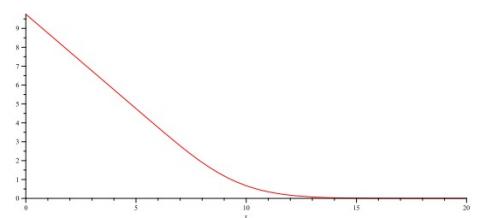
Figure 1. Exact solution at time t=T
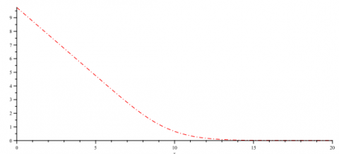
Figure 2. Approximate solution at time t=T and N=25
Figure 3. Absolute error for various N=15,20,25
The function $N(y)$ is the cumulative probability distribution function for a standardized normal distribution. Figures 1 and 2 show the exact solution and numerical solution in $t=T$ for $N=25$. The absolute error is shown for various $N=15,20,25$ in Figure 3. In Table 1, the results for N=25 for various values of S are presented in Table 1. By these results, we observe increase the accuracy of our proposed method by growing as the number of basis functions N in approximate solutions (19).
In the paper, by utilizing the backward-difference and shifted Jacobi-Galerkin method we reduce the problem to the set of system of linear algebraic equations. We also obtain the error estimation for the method. The solution obtained using the proposed technique shows that this method can solve the Black–Scholes equation for put options effectively.
[1] Stojanovic, S. (2003). Computational Financial Mathematics Using Mathematica, Optimal Trading in Stocks and Options, Springer Science, USA.
[2] Black, F., Scholes, M.S. (1973). The pricing of options and corporate liabilities. J Polit Econ, 81(3): 637-654.
[3] Fabiao, F., Grossinho, M.R., Simoes, O.A. (2009). Positive solutions of a Dirichlet problem for a stationary nonlinear Black Scholes equation. Nonlinear Analysis: Theory, Methods & Applications, 71(10): 4624-4631. https://doi.org/10.1016/j.na.2009.03.026
[4] Tangman, D.Y., Gopaul, A., Bhuruth, M. (2008). A fast high-order finite difference algorithm for pricing American options. J. Comput. Appl. Math., 222(1): 17-29. https://doi.org/10.1016/j.cam.2007.10.044
[5] Dehghan, M., Pourghanbar, S. (2011). Solution of the Black-Scholes equation for pricing of barrier option, Z. Naturforsch., A, 66(5): 289-296. https://doi.org/10.1515/zna-2011-0504
[6] Naik, P.A., Zu, J., Owolabi, K.M. (2020). Modeling the mechanics of viral kinetics under immune control during primary infection of HIV-1 with treatment in fractional order. Physica A: Statistical Mechanics and Its Applications, 545: 123816. https://doi.org/10.1016/j.physa.2019.123816
[7] Naik, P.A., Zu, J., Owolabi, K.M. (2020). Global dynamics of a fractional order model for the transmission of HIV epidemic with optimal control. Chaos Solitons Fractals, 138: 109826. https://doi.org/10.1016/j.chaos.2020.109826
[8] Naik, P.A., Zu, J., Kolade, Ghoreishi, M. (2020). Stability analysis and approximate solution of SIR epidemic model with Crowley-Martin type functional response and holling type-II treatment rate by using homotopy analysis method. J Appl Anal Comput., 10(4): 1482-1515. https://doi.org/10.11948/20190239
[9] Canuto, C., Hussaini, M.Y., Quarteroni, A., Zang, T.A. (1988). Spectral Methods in Fluid Dynamics, Springer-Verlag, New York.
[10] Mardani, A., Hooshmandasl, M.R., Heydari, M.H., Cattani, C. (2017). A meshless method for solving the time fractional advection-diffusion equation with variable coefficients. Computers & Mathematics with Applications, 75(1): 122-133. https://doi.org/10.1016/j.camwa.2017.08.038
[11] Coutsias, E.A., Hagstrom, T., Torres, D. (1996). An efficient spectral method for ordinary differential equations with rational function. Math. Comput., 65(214): 611-635.
[12] Heydari, M.H., Hooshmandasl, M.R., Maalek Ghaini, F.M., Cattani, C. (2014). A computational method for solving stochastic Ito-Volterra integral equations based on stochastic operational matrix for generalized hat basis functions. Journal of Computational Physics, 270: 402-415. https://doi.org/10.1016/j.jcp.2014.03.064
[13] Ardabili, J.S., Talaei, Y. (2018). Chelyshkov collocation method for solving the two-dimensional Fredholm-Volterra integral equations. International Journal of Applied and Computational Mathematics, 4: 25. https://doi.org/10.1007/s40819-017-0433-2
[14] Naik, P.A., Yavuz, M., Zu, J. (2020). The role of prostitution on HIV transmission with memory: A modeling approach. Alexandria Engineering Journal, 59(4): 2513-2531. https://doi.org/10.1016/j.aej.2020.04.016
[15] Naik, P.A., Zu, J., Ghoreishi, M. (2020). Estimating the approximate analytical solution of HIV viral dynamic model by using homotopy analysis method, Chaos Solitons & Fractals, 131:109500. https://doi.org/10.1016/j.chaos.2019.109500
[16] Company, R., Jodar, L., Pintos, J.R. (2009). A numerical method for European option pricing with transaction costs nonlinear equation. Mathematical and Computer Modelling, 50(5-6): 910-920. https://doi.org/10.1016/j.mcm.2009.05.019
[17] Talaei, Y., Asgari, V. (2017). An operational matrix based on Chelyshkov polynomials for solving multi-order fractional differential equations. Neural Computing and Applications, 30: 1369-1376. https://doi.org/10.1007/s00521-017-3118-1
[18] Talaei, Y. (2019). Chelyshkov collocation approach for solving linear weakly singular Volterra integral equations. Journal of Applied Mathematics and Computing, 60: 201-222. https://doi.org/10.1007/s12190-018-1209-5
[19] Guo, B.J., Shen, J., Wang, L.L. (2009). Generalized Jacobi polynomials/functions and their applications. Applied Numerical Mathematics, 59(5): 1011-1028. https://doi.org/10.1016/j.apnum.2008.04.003
[20] Jani, M., Javadi, S., Babolian, E. (2018). Bernstein dual-Petrov-Galerkin method: Application to 2D time fractional diffusion equation. Computational and Applied Mathematics, 37: 2335-2353. https://doi.org/10.1007/s40314-017-0455-8
[21] Kadalbajoo, M.K., Tripathi, L.P., Kumar, A. (2012). A cubic B-spline collocation method for a numerical solution of the generalized Black-Scholes equation. Math. Comput. Model., 55(3-4): 1483-1505. https://doi.org/10.1016/j.mcm.2011.10.040