Durwesh Jhodkar | Akhtar Khan | Kapil Gupta*
© 2021 IIETA. This article is published by IIETA and is licensed under the CC BY 4.0 license (http://creativecommons.org/licenses/by/4.0/).
OPEN ACCESS
The aim of this study is to determine the optimal combination of process parameters when machining commercially pure titanium grade 2. The unification of Multi objective optimization based on ratio analysis (MOORA) and fuzzy approach has applied to optimize the process parameters. Three process parameters i.e. cutting speed, tool overhang, and microhardness have been varied at three levels each and a total of twenty seven experiments have been conducted based on Taguchi’s L27 design of experiment technique. Cutting force, tool flank wear, and average surface roughness have been considered a machinability indicators to measure the process performance. Feed rate and depth of cut have been kept constant. Successful optimization is done and results show that machining titanium at higher cutting speed (140 m/min) and higher tool overhang length (65 mm) with medium hardness (1934 HV) results in lower cutting force, tool flank wear, and surface roughness. Outcomes of the present work reveal that the hybrid fuzzy-MOORA method is convincing enough to obtain the best process parameter combination for the best machinability while machining titanium type difficult-to-machine materials.
fuzzy, machining, hybrid optimization, surface roughness, tool wear
Optimization of manufacturing processes has been developed as a main strategy to obtain the desired process performance and product quality. Machining sector is one of the major contributors to attain the global manufacturing requirements. Most of the products undergo machining to get the required shape, size, and finish. Engineering materials have different responses when subject to machining operations. Some are soft and easily machinable, whereas some are hard and difficult-to-machine. Titanium and its alloys are very important materials for biomedical, industrial, and aerospace applications. They possess superior properties such as high strength-to-weight ratio, excellent corrosion resistance, and superior biocompatibility [1, 2]. But on the other hand, their machinability is extremely poor. Their machining, in general, results in extreme tool wear, excessive consumption of cutting fluid and energy, deteriorated part surface quality, and therefore escalated cost and environmental degradation. To address the aforementioned challenges as regards to the machining of titanium and its alloys, several attempts have been made by researchers. Machining with optimum process parameters, using green cutting fluids, employing treated tools, utilizing hybrid machining techniques such as heat and vibration assisted machining etc. have majorly been investigated [2].
As far as optimization of machining parameters is concerned, many statistical and soft computing based techniques have been developed and used to enhance the machinability of titanium and its alloys type of difficult-to-machine materials.
During turning, cutting force, surface roughness, and tool wear are the leading response variables that play a key role to achieve a low-cost product with better surface quality. It is evitable that cutting tool with lower tool wear produces good surface finish with lower cutting force as well as low tooling cost. Therefore, to attain the aforesaid objective there is a strong need of optimization technique through which the optimal combinations of cutting parameters, that affect the response variables, can be determined. Some researchers performed the statistical and prediction modeling using design of experiment (DOE) method to identify the optimum cutting parameters using various optimization techniques.
Jhodkar et al. [1] has determined the optimal cutting parameters viz. speed, feed and depth of cut using Taguchi based desirability approach for the turning of AISI 1040 steel. The authors suggested that the predicted models were best suited to optimize the machining performance of microwave treated tool inserts in terms of tool wear, cutting force and surface roughness. Ramanujam et al. [2] optimized the cutting parameters during the turning of AI-SiC(10p) using Grey relational technique. The machining performance were evaluated by surface roughness and specific power. Results revealed that the obtained optimum combination of cutting speed, feed, and depth of cut produces a good surface finish. Similarly, Yang and Tarng [3] determined the optimum cutting parameters during turning of the S45C steel bar using WC inserts to obtain better surface roughness and longer tool life. The Taguchi based optimization method employed to determine the optimum combination. Aggarwal and Singh [4] reviewed various optimization techniques for optimizing the machining parameters in turning process. In another study, the tool geometry parameters were optimized using response surface methodology during turning of AISI 1040 steel [5].
A wide range of multi-criteria decision making (MCDM) techniques such as Multi-Objective Optimization Based on Ratio Analysis (MOORA), Gray Relation Analysis (GRA), Technique for Order of Preference by similarity to Ideal Solution (TOPSIS), Taguchi Grey Relational Analysis (TGRA), Fuzzy logic, Analytical network process (ANP), and Analytical hierarchy (AHP), etc. are used for prediction and optimization of multi-attribute problems in machining [3].
Some of the important works are discussed here as under.
Tansel and Sebla [6] implemented the MOORA-based Taguchi method to solve the multi-response optimization problem for the improvement of process quality. On the other hand, Rajesh et al. [7] determined the optimal combination of wear parameters and coefficient of friction of the red mud reinforced aluminum metal matrix composite using MOORA based Taguchi method. They obtained significant improvement in wear resistance through MOORA method. Chinchanikar and Choudhury [8] evaluated the optimal cutting conditions using response surface methodology based desirability approach. Results indicated that while turning 35 and 45 HRC work material by limiting the cutting speed to 235 and 144m/min at lower feed and depth of cut, the minimum surface roughness and cutting forces with better tool life can be obtained during machining of titanium alloy.
Khan and Maity [9] studied the VIKOR based MCDM method combined with the Taguchi technique for the optimization of cutting variables to obtain the best values of surface roughness, material removal rate (MRR), and cutting force. Taguchi L27 was used for the turning of commercially pure (CP) titanium grade 2 workpiece. Results showed that cutting speed was the most influencing parameter followed by feed rate. In another important study, Khan and Maity [10] used a hybrid fuzzy-TOPSIS approach and obtained an optimal combination of cutting parameters (speed, feed, and depth of cut) that offered a significant reduction in tool wear, cutting force, and surface roughness.
During turning of medium carbon steel, Wang et al. [11] employed the hybrid fuzzy-grey optimization technique to determine uncertainty in cutting force. Results indicated that fuzzy-grey model has predicted the cutting force significantly.
Sahu and Andhare [12] performed multiobjective optimization using Teaching learning-based optimization (TLBO) and genetic algorithm (GA) during machining of Ti-6Al-4V titanium alloy. They investigated that higher cutting speed (171.4 m/min) and lower feed rate (55.6 mm/rev) produced optimal surface roughness and cutting force. In another study, Gok [13] successfully obtained the optimal cutting parameters using fuzzy TOPSIS and multi-objective grey design for surface roughness and cutting force when turning ductile iron. The depth of cut was identified as the most significant parameter.
Available literature revealed that an extensive study has been carried out to solve the multi-objective turning problems. From the literature survey, it is observed that a wide range of MCDM based optimization articles have been published which deals with multi-objective problems. However, the vague phenomenon of the cutting parameters such as cutting speed, tool microhardness and tool overhang, and output responses viz. cutting force, flank wear and surface roughness were not studied adequately using the hybrid-MCDM optimization technique so far. No article is available in which tool microhardness and tool overhang length followed by cutting speed have been considered to evaluate the optimal parametric combination during turning of CP-Ti grade 2 using MCDM based approach.
The present work fulfills the gap where cutting speed, cutting tool microhardness, and tool overhang have been considered as the input variable machining parameters while turning commercially pure titanium grade 2 (CP-Ti grade 2). Tool wear, cutting force, and surface roughness have been considered as the output parameters as machinability indicators. Before describing the optimization methodology, it’s important to mention about the two unique input parameters namely tool microhardness and overhang. The performance of the cutting tool is largely affected by tool vibration that occurs due to tool overhang length. Tool overhang length effects tool rigidity and tool vibrations that consequently affect tool wear and surface quality of the workpiece [9, 10]. Microhardness of cutting tool is also an important mechanical property and complement it to withstand adverse machining conditions [11]. Higher the microhardness, higher the tool strength will be to resist wear and failure.
In this study, the main objective is to obtain the best parametric combination of input variables using fuzzy embedded MOORA method. The hybrid MCDM based approach using fuzzy embedded MOORA method has been introduced to obtain the best parametric combination during turning of CP-Ti grade 2 using carbide tool inserts in dry cutting conditions. Taguchi’s L27 array orthogonal array has been used to design the experiments.
This section has introduced the machining of difficult-to-machine materials. It also reported some important past work on optimization of machining parameters for machinability enhancement of these materials along with summary of literature review and scope of the work presented in this paper. Next section 2 describes the optimization methodology adopted in this work. Section 3 sheds light on design of experiment technique i.e. Taguchi robust technique and experimentation strategy followed in the present work. Section 4 presents the analysis and discussion of results. Finally, section 5 concludes the paper and provides recommendation for future work.
2.1 Optimization
2.1.1 MOORA
The multi-criteria decision making based MOORA method is suitable to identify the combination of best parameters. This method was developed by Braurers and Zavadkas in the year 2004. It is used to optimize two or more conflicting objectives (criteria) subject to certain constraints [3, 6]. The reference point and ratio system are the two important elements in this method that determine the overall performance of each alternative.Ithas wide application in various sectors such as industrial sectors, manufacturing plants, banking, and insurance sectors, etc. In these aforementioned areas, multi objectives problems mostly occur where two or more conflicting attributes take place and need to identify one optimal choice [14, 15].
The proposed approach in MOORA is outlined in the following steps [3, 13]:
Step 1: MOORA method initiates with the decision matrix as shown in Equation 1 that illustrates the performance of all responses with respect to the selected input process parameters.
$P\,\,=\,\,\,\left[ \begin{matrix} {{p}_{11}} & {{p}_{12}} & ... & ... & {{p}_{1a}} \\ {{p}_{21}} & {{p}_{22}} & ... & ... & {{p}_{2b}} \\ ... & ... & ... & ... & ... \\ ... & ... & ... & ... & ... \\ {{p}_{a1}} & {{p}_{a2}} & ... & ... & {{p}_{ab}} \\\end{matrix} \right]$ (1)
where, P is a performance measure of the ith alternative on jth criterion and pij represents the output responses of the ith alternative on jth criterion, a and b are the number of alternatives and several criteria.
Step 2: The data of decision matrix gets normalized by the formation of the ration system as shown in Eq. (2).
$p_{i j}^{*}=\frac{p_{i j}}{\sqrt{\sum_{i=1}^{b} p_{i j}^{2}}}(j=1,2, \ldots \ldots, n)$ (2)
here, $p_{i j}^{*}$ represents the normalized value that lies between 0 and 1is dimensionless quantity of the i th alternative on j th criterion.
Step 3: In this step, the ranking scores are identified by MOORA index, or overall assessment values (qi) are obtained by the addition and subtraction of weighted normalized values corresponding to each alternative shown in Eq. (3). For multi-objective optimization to measure the overall assessment values benefit response (higher-is-better) are added in normalized values in case of maximization whereas in case of minimization the non-beneficial (lower-is-better) are subtracted.
$q_{i}=\sum_{j=1}^{x} p_{i j}^{*}-\sum_{j=x+1}^{y} p_{i j}^{*}$ (3)
where, x represents the number of criteria to be maximized belongs to benefit responses, whereas number of criteria is denoted by (y-x) which needs to be minimized. The normalized assessed value of i th alternative with respect to all criteria is represented by qi.
Primarily, it was observed that a few of the criteria are more essential than others. Hence, in such circumstances, the more importance is given to weight criteria and it can be multiplied with the corresponding weight. In such condition Eq. (3) would be written as Eq. (4):
$q_{i}=\sum_{j=1}^{x} r_{j} p_{i j}^{*}-\sum_{j=x+1}^{y} r_{j} p_{i j}^{*}$ (4)
where, rj is the weight of jth criteria.
Step 4: In the decision matrix, the calculated overall assessment values can be obtained positive or negative depending upon beneficial(maxima) and non-beneficial (minima) attributes. The optimal value is determined by larger MOORA value (qi) which shows the best result and the lowest value of qi represents the worst result.
2.1.2 Fuzzy set theory
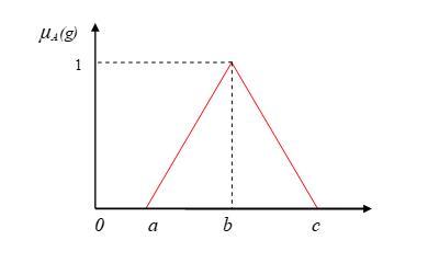
In the real-time manufacturing system, multi-criteria decision making (MCDM) related problems occur several times, due to the presence of multiple conflicting criteria. At a large scale, these problems are more complicated because of uncertain situations. In such circumstances, Fuzzy set theory helps to treat uncertainties in the form of vagueness and ambiguity to provide the best results. In the fuzzy set theory, the linguistic approach has constructed by fuzzy logic in which variables can assume linguistic values. With the help of fuzzy set theory, the opinions given by decision makers are term as specified linguistic variables. A fuzzy membership function converts aforesaid linguistic variables into a different fuzzy number. In this way, the fuzzy set theory has the ability to solve the MCDM problems effectively with ease. Fuzzy membership function can be represented in the triangular form as shown in Figure 1. Some important definitions of fuzzy numbers and fuzzy set theory are explained below [3, 16-18]:
Definition 1: A fuzzy set $\tilde{P}$ in a universe of discourse Xis described by a membership function $\mu_{\tilde{A}}(g)$ which is characterized as the grade of membership of g in $\tilde{P}$.
Figure 1. A triangular fuzzy membership function
Definition 2: $\tilde{P}$= (p1, p2, p3), are triangular fuzzy numbers (TFNs) where $\tilde{P}$ is the membership function of the fuzzy number can be written as below (Eq. (6)):
$\mu_{\tilde{A}}(g)=\left\{\begin{array}{ll}0 & g<1, \\ \frac{g-p_{1}}{p_{2}-p_{1}} & p_{1} \leq g \leq p_{2}, \\ \frac{p_{3}-g}{p_{3}-p_{2}} & p_{2} \leq g \leq a_{3}, \\ 0 & g>p_{3}\end{array}\right.$ (5)
Definition 3: The fuzzy sum and fuzzy subtraction of two different TFNs are also triangular fuzzy numbers. But, the multiplication of two different TFNs is only an approximate TFN. For example, if there are two triangular fuzzy numbers $\tilde{P}=\left(p_{1}, p_{2}, p_{3}\right)$ and $\tilde{Q}=\left(q_{1}, q_{2}, q_{3}\right)$, and a positive real number w = (w, w, w), some important operations of fuzzy numbers can be written as follows:
$\tilde{P}(+) \tilde{Q}=\left(p_{1}+p_{2}, q_{1}+p_{2}, q_{1}+r_{2}\right)$ (6)
$\tilde{P}(-) \tilde{Q}=\left(p_{1}-p_{2}, q_{1}-q_{2}, r_{1}-r_{2}\right)$ (7)
$\tilde{P}(\times) \tilde{Q}=\left(p_{1} p_{2}, q_{1} q_{2}, r_{1} r_{2}\right)$ (8)
$\tilde{P}(/) \tilde{Q}=\left(p_{1} / q_{1}, p_{2} / q_{2}, p_{3} / q_{3}\right)$ (9)
$\tilde{P}(\times) w=\left(p_{1} w, p_{2} w, p_{3} w\right)$ (10)
Definition 4: A triangular fuzzy number $\tilde{P}=\left(p_{1}, p_{2}, p_{3}\right)$, then the defuzzified value $a(\tilde{P})$ can be determined using Eq. (11):
$a(\tilde{P})=\frac{p_{1}+p_{2}+p_{3}}{3}$ (11)
Definition 5: The two triangular fuzzy numbers are $\tilde{P}=\left(p_{1}, p_{2}, p_{3}\right)$ and $\tilde{Q}=\left(q_{1}, q_{2}, q_{3}\right)$, and the distance between $(\tilde{P})$ and $(\tilde{Q})$ can be computed using Eq. (12):
$d(\tilde{P}, \tilde{Q})=\sqrt{\frac{1}{3}\left(p_{1}-q_{1}\right)^{2}+\left(p_{2}-q_{2}\right)^{2}+\left(p_{3}-q_{3}\right)^{2}}$ (12)
Definition 6: By applying center of area approach, the best non-fuzzy performance (BNP) value can be determined and expressed as Eq. (13):
$B N P_{i}=\frac{[(r-p)+(q-p)]}{3}+p, \forall_{i}$ (13)
2.1.3 Fuzzy embedded MOORA method
The extension of the MOORA method is a systematic approach to solve the multi-criteria decision making in the fuzzy environment. Various researchers of real-time manufacturing attempted the hybridization of two approaches. Hence, this hybrid approach used to identify optimal parametric combinations to confirm improvement in the machining performance of WC cutting tool inserts. In this hybrid fuzzy-MOORA method, the opinions of decision-makers express in the terms of a set of linguistic variables. The fuzzy embedded MOORA method followed by the following steps:
Step 1: Between all alternatives(rows) and criteria (columns) the fuzzy decision matrix has been formed that belong to fuzzy triangular numbers as shown in Eq. (14)
$\tilde{P}=\left[\begin{array}{ccc}{\left[p_{11}^{a}, p_{11}^{b}, p_{11}^{c}\right]} & {\left[p_{12}^{a}, p_{12}^{b}, p_{12}^{c}\right]} & {\left[p_{1 c}^{a}, p_{1 c}^{b}, p_{1 c}^{c}\right]} \\ \ldots & \cdots & \ldots \\ {\left[p_{b 1}^{a}, p_{b 1}^{b}, p_{b 1}^{c}\right]} & p_{b 2}^{a}, p_{b 2}^{b}, p_{b 2}^{c} & p_{b c}^{a}, p_{b c}^{b}, p_{b c}^{c}\end{array}\right]$ (14)
Step 2: Using Eqns. (15-17), the normalized fuzzy decision matrix has been calculated
$p_{i j}^{a^{*}}=\frac{p_{i j}^{a}}{\sqrt{\sum_{i=1}^{b}\left[\left(p_{i j}^{a}\right)^{2}+\left(p_{i j}^{b}\right)^{2}+\left(p_{i j}^{c}\right)^{2}\right]}}$ (15)
$p_{i j}^{b^{*}}=\frac{p_{i j}^{b}}{\sqrt{\sum_{i=1}^{m}\left[\left(p_{i j}^{a}\right)^{2}+\left(p_{i j}^{b}\right)^{2}+\left(p_{i j}^{c}\right)^{2}\right]}}$ (16)
$p_{i j}^{c^{*}}=\frac{p_{i j}^{c}}{\sqrt{\sum_{i=1}^{b}\left[\left(p_{i j}^{a}\right)^{2}+\left(p_{i j}^{b}\right)^{2}+\left(p_{i j}^{c}\right)^{2}\right]}}$ (17)
Step 3: Calculate the weighted normalized fuzzy decision matrix using Eqns. (18-20).
$W_{i j}^{a}=r_{j} p_{i j}^{a^{*}}$ (18)
$W_{i j}^{b}=r_{j} p_{i j}^{b *}$ (19)
$W_{i j}^{c}=r_{j} p_{i j}^{c *}$ (20)
rj is the weight criteria of each attribute in aforesaid equations.
Step 4: The non-fuzzy value(crisp) has converted from overall fuzzy assessment value $\left(\tilde{q}_{i}\right)$. Eq. (21) can be used to calculate the best non-fuzzy performance (BNP) as expressed below:
$B N P_{i}\left(q_{i}\right)=\frac{\left(q_{i}^{c}-q_{i}^{a}\right)+\left(q_{i}^{b}-q_{i}^{a}\right)}{3}+q_{i}^{a}$ (21)
where, $\tilde{q}_{i}=\left(q_{i}^{a}, q_{i}^{b}, q_{i}^{c}\right)$.
Step 5: In this step the overall fuzzy assessment value can be computed by applying Eq. (22).
$\tilde{q}_{i}=\tilde{W}_{i j}^{+}-\tilde{W}_{i j}^{-}$ (22)
$\widetilde{W}_{i j}^{+}$ and $\widetilde{W}_{i j}^{-}$ are overall assessment value of beneficial and non-beneficial criteria respectively.
Step 6: Allocate ranking to all the computed closeness values in descending order. In which the best alternative refer by higher closeness value that indicates the best performance, and vice versa.
3.1 Design of experiment
3.1.1 Taguchi technique
Taguchi’s optimization method has wide applications to minimize the number of experiment trials without affecting the quality of results [19]. Taguchi recommended a three-stage process (a) system design (b) parameter design (c) tolerance [20, 21]. In system design, the optimum condition and working levels of design parameters are identified which affects the minimum variation to system performance. Whereas, in parameter design, the levels of the parameters are selected that result in the best performance of the process during experiments. Signal to the noise ratio analysis, variance study, and orthogonal arrays are important tools used for parameter design [22]. In tolerance design, the selected parameters that influence outcome of the process product are finely tuned by tightening the tolerance of parameters [21, 23].
Table 1. Input machining parameters and levels
|
S No. |
Parameters |
Units |
Levels |
||
|
Low |
Medium |
High |
|||
|
1. |
Cutting speed |
m/min |
50 |
95 |
140 |
|
2. |
Microhardness (Avg) |
HV |
1689 |
1934 |
2307 |
|
3. |
Tool overhang |
mm |
25 |
45 |
65 |
Table 2. Experimental combinations and responses
|
Run |
Input parameters |
Responses |
||||
|
A (m/min) |
B (HV) |
C (mm) |
Fc (N) |
VBc (mm) |
Ra (µm) |
|
|
1 |
50 |
1689 |
25 |
69.31 |
0.136 |
2.27 |
|
2 |
50 |
1689 |
45 |
117.43 |
0.154 |
2.48 |
|
3 |
50 |
1689 |
65 |
101.48 |
0.277 |
2.71 |
|
4 |
50 |
1934 |
25 |
137.49 |
0.158 |
2.55 |
|
5 |
50 |
1934 |
45 |
112.53 |
0.141 |
2.45 |
|
6 |
50 |
1934 |
65 |
80.50 |
0.286 |
2.75 |
|
7 |
50 |
2307 |
25 |
128.48 |
0.153 |
3.12 |
|
8 |
50 |
2307 |
45 |
80.10 |
0.153 |
2.85 |
|
9 |
50 |
2307 |
65 |
98.53 |
0.220 |
3.19 |
|
10 |
95 |
1689 |
25 |
78.65 |
0.248 |
2.47 |
|
11 |
95 |
1689 |
45 |
118.97 |
0.295 |
2.49 |
|
12 |
95 |
1689 |
65 |
103.08 |
0.279 |
2.58 |
|
13 |
95 |
1934 |
25 |
155.29 |
0.211 |
2.80 |
|
14 |
95 |
1934 |
45 |
114.73 |
0.147 |
2.77 |
|
15 |
95 |
1934 |
65 |
70.61 |
0.284 |
2.67 |
|
16 |
95 |
2307 |
25 |
131.14 |
0.200 |
2.85 |
|
17 |
95 |
2307 |
45 |
81.73 |
0.165 |
3.25 |
|
18 |
95 |
2307 |
65 |
99.79 |
0.250 |
2.97 |
|
19 |
140 |
1689 |
25 |
79.66 |
0.164 |
1.79 |
|
20 |
140 |
1689 |
45 |
120.81 |
0.178 |
1.87 |
|
21 |
140 |
1689 |
65 |
104.53 |
0.222 |
1.85 |
|
22 |
140 |
1934 |
25 |
141.28 |
0.082 |
2.15 |
|
23 |
140 |
1934 |
45 |
115.80 |
0.157 |
1.79 |
|
24 |
140 |
1934 |
65 |
72.40 |
0.171 |
1.57 |
|
25 |
140 |
2307 |
25 |
131.93 |
0.165 |
2.02 |
|
26 |
140 |
2307 |
45 |
86.37 |
0.179 |
2.09 |
|
27 |
140 |
2307 |
65 |
101.91 |
0.193 |
1.96 |
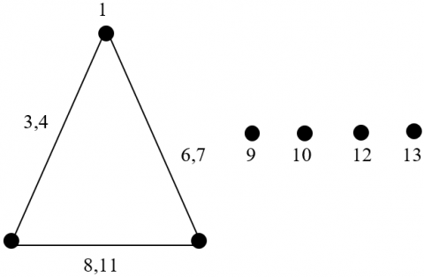
In the current study, three levels viz low, medium and high of each process parameter were analyzed because the nonlinear behavior among the process parameters, if exists, can only be revealed if more than two levels of the parameters are investigated. Three input variable parameters viz. cutting speed (v), microhardness hardness (m), and tool overhang length (l)with their three levels are given in Table 1. In the experiment, the total degree of freedom (DOF) calculated is 18 because of three parameters at three levels and three second-order interactions. Three parameters have two degree of freedom (N-1) and each second-order interaction has four degree of freedom. Therefore, [3 × (3-1)+3× (2×2) =18]. According to the Taguchi‘s technique, the selected orthogonal array (OA) and its total degree of freedom must be greater than or equal to the total degree of freedom required for the experiment. Therefore, in this study, Taguchi’s robust technique with L27 (33) orthogonal array which having 26 degree of freedom has been used to design experiments. The process parameters were allocated according to the linear graph shown in Figure 2. Each experiment was performed for a fixed duration in order to remove the biasedness. All twenty-seven experimental combinations/settings with corresponding values of output parameters i.e. cutting force (Fc), tool flank wear (VBc), and average surface roughness (Ra) are listed in Table 2.
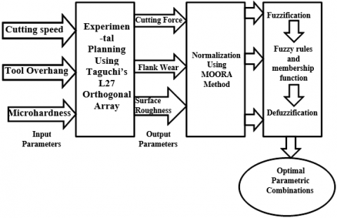
Figure 3 illustrates the process flow chart of the methodology adopted in this study to obtain optimal combination using fuzzy-MOORA hybrid method.
Figure 2. Linear graph of L27 orthogonal array (OA)
Figure 3. Process flow chart presents the methodology
3.2 Experimental procedure
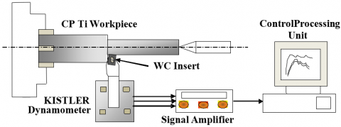
Turning experiments have been performed on a heavy duty H.M.T lathe to machine commercial pure (CP) titanium alloy grade 2 having a diameter of 60 mm and length of 500 mm. The chemical compositions of workpiece are Carbon 0.08-0.1%, Nitrogen 0.03-0.05, Oxygen 0.25%(max), Iron (Fe) 0.30%, Hydrogen 0.015%, Titanium balance% and others 0.4%. Square-shaped uncoated tungsten carbide (WC) tool inserts SNMG 120408 manufactured by Kennametal have been used for machining. Figure 4 presents the schematic representation of the experimental setup used in the present work.
Figure 4. Schematic of the experimental setup used in the present work
In this study, the microwave treatment is done on cutting tool inserts in order to vary the tool microhardness. The microhardness variation is as follows:
Microhardness (HV) of WC tool inserts untreated- 1689 HV, Microhardness (HV) of WC tool inserts 20 min treated- 1934 HV, Microhardness (HV) of WC tool inserts 30 min treated 2307 HV. The levels of cutting speed, and constant values of feed and depth of cut have been selected based on literature review, machine constraints, and tool manufacturer’s recommendation. Cutting force (Fc), flank wear (VBc), and Surface roughness (Ra.) were selected as output responses to assess the performance. After each turning operation/experiment, tool inserts were removed from tool holder for the offline measurement of flank were (Vb) under Axio Cam USB microscope. At four different places of workpiece, average surface roughness (Ra) was measured by Taylor Hobson surface roughness tester, and theaverage value was considered. KISTLER (Type 9257A) three-component piezoelectric dynamometer was used to measure the cutting force.
4.1 FUZZY-MOORA based optimum parameters
In the present research work, the best parametric combination of input variables was determined during the machining of CP-Ti grade 2 using fuzzy embedded MOORA method. The objective was to minimize the tool wear, cutting force, and surface roughness. The interaction effects between the complexness of machining characteristics and process parameters create difficulties to recommend the best parametric combinations during machining.
When the decision-maker faces troubles to express quantitative values and dealing with situations that are too ill-defined and complex, in such conditions, decision-maker uses the non-numerical form in words known as linguistic terms such as excellent, good, very good, low, very low, poor etc., to express values in the qualitative thoughts of the prepared workpiece [24]. Therefore, selecting the optimum among the available parameters is a challenging task. Assessment of machining parameters of all alternatives i.e. very poor, poor, average, very good etc. with their triangular fuzzy numbers are shown in Table 3. The aforesaid linguistic variables are represented by triangular fuzzy numbers. The first linguistic variable (very very low) having TFN 0,0,0.1 whereas the last linguistic variables (very very high) of Table 3 having TFN (0.9, 1.0, 1.0), Therefore, the assigned triangular fuzzy numbers lie between 0 to 1.
Furthermore, mentioned linguistics variables and triangular fuzzy numbers are used to express the relative weight of each machining response. The specified linguistic variables were obtained by the relative weight of selected output responses such as flank wear, cutting force, and surface roughness as shown in Table 4. Tool wear is an unavoidable phenomenon during machining and it affects the cutting force and surface roughness of the workpiece. Therefore, relative weight for tool wear is kept at very very high (VVH) priority in Table 4 as compared to the cutting force and surface roughness. Whereas, cutting force and surface roughness are also essential criteria during machining are given relative weight very high (VH). The corresponding triangular fuzzy number values of criteria (Table 4) are referred from linguistic variables values of Table 3.
Furthermore, all the available alternatives were evaluated and validated based on linguistic variables. The values of triangular fuzzy nubers for linguistic variables are lied between 0 to 10. The seven different fuzzy linguistics variables such as very very good (VVG), very good (VG) good (G) fair (F), poor (P), very poor (VP) and very very poor (VVP) were obtained during the valuation as shown in Table 5.
Table 3. Linguistic variables used for each criterion
|
Linguistic variable |
Triangular fuzzy numbers (TFNs) |
|
Very very low (VVL) |
(0, 0, 0.1) |
|
Very low (VL) |
(0, 0.1, 0.3) |
|
Low (L) |
(0.1, 0.3, 0.5) |
|
Medium (M) |
(0.3, 0.5, 0.7) |
|
High (H) |
(0.5, 0.7, 0.9) |
|
Very high (VH) |
(0.7, 0.9, 1.0) |
|
Very very high (VVH) |
(0.9, 1.0, 1.0) |
Table 4. Relative weights of each criterion
|
Criteria |
Decision maker |
Fuzzy numbers |
|
Fc |
VH |
(0.7, 0.9, 1.0) |
|
VBc |
VVH |
(0.9, 1.0, 1.0) |
|
Ra |
VH |
(0.7, 0.9, 1.0) |
Table 5. Linguistic variables used for each alternative
|
Linguistic variable |
Triangular fuzzy numbers (TFNs) |
|
Very very poor (VVP) |
(0, 0, 1) |
|
Very poor (VP) |
(0, 1, 3) |
|
Poor (P) |
(1, 3, 5) |
|
Fair (F) |
(3, 5, 7) |
|
Good (G) |
(5, 7, 9) |
|
Very good (VG) |
(7, 9, 10) |
|
Very very good (VVG) |
(9, 10, 10) |
Table 6. Results of the assessment
|
Altern-atives |
Output responses |
Fuzzy linguistic variables |
||||
|
Fc |
VBc |
Ra |
Fc |
VBc |
Ra |
|
|
1 |
69.31 |
0.136 |
2.27 |
VVG |
VG |
G |
|
2 |
117.43 |
0.154 |
2.48 |
F |
G |
F |
|
3 |
101.48 |
0.277 |
2.71 |
G |
VVP |
P |
|
4 |
137.49 |
0.158 |
2.55 |
VP |
G |
P |
|
5 |
112.53 |
0.141 |
2.45 |
F |
VG |
F |
|
6 |
80.50 |
0.286 |
2.75 |
VVG |
VVP |
P |
|
7 |
128.48 |
0.153 |
3.12 |
P |
G |
VVP |
|
8 |
80.10 |
0.153 |
2.85 |
VVG |
G |
VP |
|
9 |
98.53 |
0.220 |
3.19 |
G |
P |
VVP |
|
10 |
78.65 |
0.248 |
2.47 |
VVG |
VP |
F |
|
11 |
118.97 |
0.295 |
2.49 |
P |
VVP |
F |
|
12 |
103.08 |
0.279 |
2.58 |
G |
VVP |
P |
|
13 |
155.29 |
0.211 |
2.80 |
VVP |
P |
VP |
|
14 |
114.73 |
0.147 |
2.77 |
F |
G |
VP |
|
15 |
70.61 |
0.284 |
2.67 |
VVG |
VVP |
P |
|
16 |
131.14 |
0.200 |
2.85 |
VP |
F |
VP |
|
17 |
81.73 |
0.165 |
3.25 |
VG |
G |
VVP |
|
18 |
99.79 |
0.250 |
2.97 |
G |
VP |
VP |
|
19 |
79.66 |
0.164 |
1.79 |
VVG |
G |
VVG |
|
20 |
120.81 |
0.178 |
1.87 |
P |
F |
VG |
|
21 |
104.53 |
0.222 |
1.85 |
G |
P |
VG |
|
22 |
141.28 |
0.082 |
2.15 |
VP |
VVG |
G |
|
23 |
115.80 |
0.157 |
1.79 |
F |
G |
VVG |
|
24 |
72.40 |
0.171 |
1.57 |
VVG |
G |
VVG |
|
25 |
131.93 |
0.165 |
2.02 |
VP |
G |
VG |
|
26 |
86.37 |
0.179 |
2.09 |
VG |
F |
G |
|
27 |
101.91 |
0.193 |
1.96 |
G |
F |
VG |
Furthrmore, aforementioned fuzzy linguistics variables have assigned to 27 alternatives to achive the best combination (refer Table 6). All crips values of output responses (Fc,VBc and Ra) converted into the linguistic variables according to the prirority. For example, the range of lowest tool wear (0.082 mm) has denoted by very very good (VVG) and higher tool wear (0.277-0.295 mm) have denoted by very very poor (VVP). The assessment of the results is shown in Table 6. The output responses viz. flank wear, cutting force, and surface roughness are represented into fuzzy linguistics variables. After this, suitable triangular fuzzy numbers were prepared by the formation of a fuzzy decision matrix that is done by converting the data sets obtained after assessment.
Table 7. Fuzzy decision matrix
|
Alternative |
Responses |
||
|
Fc |
VBc |
Ra |
|
|
1 |
9, 10, 10 |
7, 9, 10 |
5, 7, 9 |
|
2 |
3, 5, 7 |
5, 7, 9 |
3, 5, 7 |
|
3 |
5, 7, 9 |
0, 0, 1 |
1, 3, 5 |
|
4 |
0, 1, 3 |
5, 7, 9 |
1, 3, 5 |
|
5 |
3, 5, 7 |
7, 9, 10 |
3, 5, 7 |
|
6 |
9, 10, 10 |
0, 0, 1 |
1, 3, 5 |
|
7 |
1, 3, 5 |
5, 7, 9 |
0, 0, 1 |
|
8 |
9, 10, 10 |
5, 7, 9 |
0, 1, 3 |
|
9 |
5, 7, 9 |
1, 3, 5 |
0, 0, 1 |
|
10 |
9, 10, 10 |
0, 1, 3 |
3, 5, 7 |
|
11 |
1, 3, 5 |
0, 0, 1 |
3, 5, 7 |
|
12 |
5, 7, 9 |
0, 0, 1 |
1, 3, 5 |
|
13 |
0, 0, 1 |
1, 3, 5 |
0, 1, 3 |
|
14 |
3, 5, 7 |
5, 7, 9 |
0, 1, 3 |
|
15 |
9, 10, 10 |
0, 0, 1 |
1, 3, 5 |
|
16 |
0, 1, 3 |
3, 5, 7 |
0, 1, 3 |
|
17 |
7, 9, 10 |
5, 7, 9 |
0, 0, 1 |
|
18 |
5, 7, 9 |
0, 1, 3 |
0, 1, 3 |
|
19 |
9, 10, 10 |
5, 7, 9 |
9, 10, 10 |
|
20 |
1, 3, 5 |
3, 5, 7 |
7, 9, 10 |
|
21 |
5, 7, 9 |
1, 3, 5 |
7, 9, 10 |
|
22 |
0, 1, 3 |
9, 10, 10 |
5, 7, 9 |
|
23 |
3, 5, 7 |
5, 7, 9 |
9, 10, 10 |
|
24 |
9, 10, 10 |
5, 7, 9 |
9, 10, 10 |
|
25 |
0, 1, 3 |
5, 7, 9 |
7, 9, 10 |
|
26 |
7, 9, 10 |
3, 5, 7 |
5, 7, 9 |
|
27 |
5, 7, 9 |
3, 5, 7 |
7, 9, 10 |
Table 8. Normalized fuzzy decision matrix
|
Alter-natives |
Responses |
||
|
Fc |
VBc |
Ra |
|
|
1 |
0.9, 0.1, 0.1 |
0.7, 0.9, 0.1 |
0.5, 0.7, 0.9 |
|
2 |
0.3, 0.5, 0.7 |
0.5, 0.7, 0.9 |
0.3, 0.5, 0.7 |
|
3 |
0.5, 0.7, 0.9 |
0, 0, 0.1 |
0.1, 0.3, 0.5 |
|
4 |
0, 0.1, 0.3 |
0.5, 0.7, 0.9 |
0.1, 0.3, 0.5 |
|
5 |
0.3, 0.5, 0.7 |
0.7, 0.9, 0.1 |
0.3, 0.5, 0.7 |
|
6 |
0.9, 0.1, 0.1 |
0, 0, 0.1 |
0.1, 0.3, 0.5 |
|
7 |
0.1, 0.3, 0.5 |
0.5, 0.7, 0.9 |
0, 0, 0.1 |
|
8 |
0.9, 0.1, 0.1 |
0.5, 0.7, 0.9 |
0, 0.1, 0.3 |
|
9 |
0.5, 0.7, 0.9 |
0.1, 0.3, 0.5 |
0, 0, 0.1 |
|
10 |
0.9, 0.1, 0.1 |
0, 0.1, 0.3 |
0.3, 0.5, 0.7 |
|
11 |
0.1, 0.3, 0.5 |
0, 0, 0.1 |
0.3, 0.5, 0.7 |
|
12 |
0.5, 0.7, 0.9 |
0, 0, 0.1 |
0.1, 0.3, 0.5 |
|
13 |
0, 0, 0.1 |
0.1, 0.3, 0.5 |
0, 0.1, 0.3 |
|
14 |
0.3, 0.5, 0.7 |
0.5, 0.7, 0.9 |
0, 0.1, 0.3 |
|
15 |
0.9, 0.1, 0.1 |
0, 0, 0.1 |
0.1, 0.3, 0.5 |
|
16 |
0, 0.1, 0.3 |
0.3, 0.5, 0.7 |
0, 0.1, 0.3 |
|
17 |
0.7, 0.9, 0.1 |
0.5, 0.7, 0.9 |
0, 0, 0.1 |
|
18 |
0.5, 0.7, 0.9 |
0, 0.1, 0.3 |
0, 0.1, 0.3 |
|
19 |
0.9, 0.1, 0.1 |
0.5, 0.7, 0.9 |
0.9, 0.1, 0.1 |
|
20 |
0.1, 0.3, 0.5 |
0.3, 0.5, 0.7 |
0.7, 0.9, 0.1 |
|
21 |
0.5, 0.7, 0.9 |
0.1, 0.3, 0.5 |
0.7, 0.9, 0.1 |
|
22 |
0, 0.1, 0.3 |
0.9, 0.1, 0.1 |
0.5, 0.7, 0.9 |
|
23 |
0.3, 0.5, 0.7 |
0.5, 0.7, 0.9 |
0.9, 0.1, 0.1 |
|
24 |
0.9, 0.1, 0.1 |
0.5, 0.7, 0.9 |
0.9, 0.1, 0.1 |
|
25 |
0, 0.1, 0.3 |
0.5, 0.7, 0.9 |
0.7, 0.9, 0.1 |
|
26 |
0.7, 0.9, 0.1 |
0.3, 0.5, 0.7 |
0.5, 0.7, 0.9 |
|
27 |
0.5, 0.7, 0.9 |
0.3, 0.5, 0.7 |
0.7, 0.9, 0.1 |
Table 9. Weighted normalized fuzzy decision matrix
|
Alter- natives |
Responses |
||
|
Fc |
VBc |
Ra |
|
|
1 |
0.63, 0.9, 0.1 |
0.63, 0.9, 0.1 |
0.35, 0.63, 0.9 |
|
2 |
0.21, 0.45, 0.7 |
0.45, 0.7, 0.9 |
0.21, 0.45, 0.7 |
|
3 |
0.35, 0.63, 0.9 |
0, 0, 0.1 |
0.7, 0.27, 0.5 |
|
4 |
0, 0.9, 0.3 |
0.45, 0.7, 0.9 |
0.7, 0.27, 0.5 |
|
5 |
0.21, 0.45, 0.7 |
0.63, 0.9, 0.1 |
0.21, 0.45, 0.7 |
|
6 |
0.63, 0.9, 0.1 |
0, 0, 0.1 |
0.7, 0.27, 0.5 |
|
7 |
0.7, 0.27, 0.5 |
0.45, 0.7, 0.9 |
0, 0, 0.1 |
|
8 |
0.63, 0.9, 0.1 |
0.45, 0.7, 0.9 |
0, 0.9, 0.3 |
|
9 |
0.35, 0.63, 0.9 |
0.9, 0.3, 0.5 |
0, 0, 0.1 |
|
10 |
0.63, 0.9, 0.1 |
0, 0.1, 0.3 |
0.21, 0.45, 0.7 |
|
11 |
0.7, 0.27, 0.5 |
0, 0, 0.1 |
0.21, 0.45, 0.7 |
|
12 |
0.35, 0.63, 0.9 |
0, 0, 0.1 |
0.7, 0.27, 0.5 |
|
13 |
0, 0, 0.1 |
0.9, 0.3, 0.5 |
0, 0.9, 0.3 |
|
14 |
0.21, 0.45, 0.7 |
0.45, 0.7, 0.9 |
0, 0.9, 0.3 |
|
15 |
0.63, 0.9, 0.1 |
0, 0, 0.1 |
0.7, 0.27, 0.5 |
|
16 |
0, 0.9, 0.3 |
0.27, 0.5, 0.7 |
0, 0.9, 0.3 |
|
17 |
0.49, 0.81, 0.1 |
0.45, 0.7, 0.9 |
0, 0, 0.1 |
|
18 |
0.35, 0.63, 0.9 |
0, 0.1, 0.3 |
0, 0.9, 0.3 |
|
19 |
0.63, 0.9, 0.1 |
0.45, 0.7, 0.9 |
0.63, 0.9, 0.1 |
|
20 |
0.7, 0.27, 0.5 |
0.27, 0.5, 0.7 |
0.49, 0.81, 0.1 |
|
21 |
0.35, 0.63, 0.9 |
0.9, 0.3, 0.5 |
0.49, 0.81, 0.1 |
|
22 |
0, 0.9, 0.3 |
0.81, 0.1, 0.1 |
0.35, 0.63, 0.9 |
|
23 |
0.21, 0.45, 0.7 |
0.45, 0.7, 0.9 |
0.63, 0.9, 0.1 |
|
24 |
0.63, 0.9, 0.1 |
0.45, 0.7, 0.9 |
0.63, 0.9, 0.1 |
|
25 |
0, 0.9, 0.3 |
0.45, 0.7, 0.9 |
0.49, 0.81, 0.1 |
|
26 |
0.49, 0.81, 0.1 |
0.27, 0.5, 0.7 |
0.35, 0.63, 0.9 |
|
27 |
0.35, 0.63, 0.9 |
0.27, 0.5, 0.7 |
0.49, 0.81, 0.1 |
The triangular fuzzy numbers of fuzzy decision matrix shown in Table 7 are obtained after conversion of linguistics variables of cutting force (Fc), tool wear (VBc), and surface roughness (Ra) of Table 6. For example, the linguistic variable very very good (VVG) (refer to Table 5) having a triangular fuzzy number (9.10,10). Therefore, all places in Table 6 the VVG is replaced by (9,10,10) in Table 7.
The fuzzy decision matrix as shown in Table 7 was implemented using Eqns. (16-18) and the results are shown in Table 8 as a normalized fuzzy decision matrix. The fuzzy decision matrix has obtained by dividing all values of Table 7 by ten (10). Afterward, Table 9 expresses a weighted normalized fuzzy decision matrix, in which the relevant weight of every machining criterion was multiplied with their adjacent values. For example, the relative weight of flank wear is very very high (VVH) whereas the relative weights of cutting force and surface roughness are very high (VH) (refer Table 3). Therefore, adjacent values of relative weights multiplied by values of normalized fuzzy decision matrix values. After that applying Eq. (22) the listed values of Table 9 further converted into crisps values are represented in Table 10.
At last, Table 11 has been developed using Eq. (23) in which complete assessment of values. For example, assessment value (yi) of alternative 1, (row 1) is calculated by the addition of consecutive crips values (refer Table 10) of cutting force (Fc), flank wear (VBc), and surface roughness (Ra). The overall assessment values have been shown in decreasing order according to the preference ranking. The highest assessment values would be denoted by rank 1 whereas the lowest assessment value would be denoted by rank 27 because total twenty-seven experiments were conducted to obtain the best parametric combination.
The experiment number 24 has been observed the best operating parameter that gives optimum responses showing less flank wear, cutting force, and surface roughness. Whereas experiment number 11 has shown the worst responses, in which flank wear, cutting force, and surface roughness has the highest values.
Table 10. Crisp values for weighted normalized fuzzy decision matrix
|
Alternative |
Responses |
||
|
Fc |
VBc |
Ra |
|
|
1 |
0.543 |
0.543 |
0.627 |
|
2 |
0.453 |
0.683 |
0.453 |
|
3 |
0.627 |
0.033 |
0.490 |
|
4 |
0.400 |
0.683 |
0.490 |
|
5 |
0.453 |
0.543 |
0.453 |
|
6 |
0.543 |
0.033 |
0.490 |
|
7 |
0.490 |
0.683 |
0.033 |
|
8 |
0.543 |
0.683 |
0.400 |
|
9 |
0.627 |
0.567 |
0.033 |
|
10 |
0.543 |
0.133 |
0.453 |
|
11 |
0.490 |
0.033 |
0.453 |
|
12 |
0.627 |
0.033 |
0.490 |
|
13 |
0.033 |
0.567 |
0.400 |
|
14 |
0.453 |
0.683 |
0.400 |
|
15 |
0.543 |
0.033 |
0.490 |
|
16 |
0.400 |
0.490 |
0.400 |
|
17 |
0.467 |
0.683 |
0.033 |
|
18 |
0.627 |
0.133 |
0.400 |
|
19 |
0.543 |
0.683 |
0.543 |
|
20 |
0.490 |
0.490 |
0.467 |
|
21 |
0.627 |
0.567 |
0.467 |
|
22 |
0.400 |
0.337 |
0.627 |
|
23 |
0.453 |
0.683 |
0.543 |
|
24 |
0.543 |
0.683 |
0.543 |
|
25 |
0.400 |
0.683 |
0.467 |
|
26 |
0.467 |
0.490 |
0.627 |
|
27 |
0.627 |
0.490 |
0.467 |
Table 11. Overall assessment value
|
Alter-natives |
Responses |
|
|||
|
Fc |
VBc |
Ra |
yi |
Rank |
|
|
1 |
0.543 |
0.543 |
0.627 |
1.713 |
3 |
|
2 |
0.453 |
0.683 |
0.453 |
1.590 |
7 |
|
3 |
0.627 |
0.033 |
0.490 |
1.140 |
22 |
|
4 |
0.400 |
0.683 |
0.490 |
1.573 |
10 |
|
5 |
0.453 |
0.543 |
0.453 |
1.450 |
13 |
|
6 |
0.543 |
0.033 |
0.490 |
1.067 |
24 |
|
7 |
0.490 |
0.683 |
0.033 |
1.207 |
18 |
|
8 |
0.543 |
0.683 |
0.400 |
1.627 |
6 |
|
9 |
0.627 |
0.567 |
0.033 |
1.227 |
17 |
|
10 |
0.543 |
0.133 |
0.453 |
1.130 |
23 |
|
11 |
0.490 |
0.033 |
0.453 |
0.977 |
27 |
|
12 |
0.627 |
0.033 |
0.490 |
1.150 |
21 |
|
13 |
0.033 |
0.567 |
0.400 |
1.000 |
26 |
|
14 |
0.453 |
0.683 |
0.400 |
1.537 |
12 |
|
15 |
0.543 |
0.033 |
0.490 |
1.047 |
25 |
|
16 |
0.400 |
0.490 |
0.400 |
1.290 |
16 |
|
17 |
0.467 |
0.683 |
0.033 |
1.183 |
19 |
|
18 |
0.627 |
0.133 |
0.400 |
1.160 |
20 |
|
19 |
0.543 |
0.683 |
0.543 |
1.761 |
2 |
|
20 |
0.490 |
0.490 |
0.467 |
1.447 |
14 |
|
21 |
0.627 |
0.567 |
0.467 |
1.660 |
5 |
|
22 |
0.400 |
0.337 |
0.627 |
1.363 |
15 |
|
23 |
0.453 |
0.683 |
0.543 |
1.680 |
4 |
|
24 |
0.543 |
0.683 |
0.543 |
1.770 |
1 |
|
25 |
0.400 |
0.683 |
0.467 |
1.550 |
11 |
|
26 |
0.467 |
0.490 |
0.627 |
1.584 |
9 |
|
27 |
0.627 |
0.490 |
0.467 |
1.583 |
8 |
Therefore, results show that at higher cutting speed (140 m/min) and higher tool overhang length (65mm) with medium hardness (1934 HV) level, the tool wear recorded less with less cutting force and good surface roughness.
The aforementioned combination reported suitable and optimum for the machining, out of 27 experiments. With the increase in the cutting speed during machining of titanium alloys the cutting temperature also rises at shear zone due to friction during turning. The high temperature at the tool-workpiece interface remains high enough to influence the surface roughness of the workpiece. This high temperature allows regenerating the workpiece surface due to thermal expansion that results in the disappearance of micro cracks and cavities from the surface of the workpiece [25].
Experiment number 24 also depicted that increase in average microhardness reduces the cutting force and flank wear significantly, however, a high level of tool overhang length does not impact surface roughness and flank wear significantly. Therefore, a higher range of machining parameters considered in this study are fairly recommended for the machining of CP-Ti grade to titanium alloy.
4.2 Analysis of results
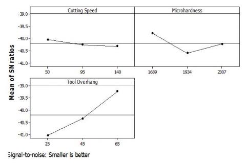
The main effect plots for cutting force, flank wear, and surface roughness are illustrated in Figures 5, 6, and 7 respectively. In Figure 5, It is depicted that cutting speed and tool overhang significantly affect the cutting force and its least value is obtained at the middle level of microhardness.
Figure 5. Main effect plot for cutting force (Fc)
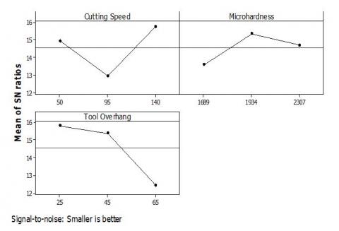
Figure 6. Main effect plot for tool flank wear (VBc)
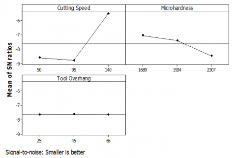
Figure 7. Main effect plot for Surface roughness (Ra)
From Figure 6, it is observed that microhardness and cutting speed play a significant role in flank wear because higher the cutting speed results in higher tool deformation and cutting temperature. However, an increase in microhardness results in an increase in wear resistance and cutting edge stability.
Figure 7 shows the main effect plot for surface roughness, it is observed that cutting speed, microhardness, and tool overhang are significantly affecting the surface roughness. At lower cutting speed, surface roughness is higher, whereas at higher cutting speed, the surface roughness is observed lower due to regeneration of the workpiece surface at a higher cutting temperature [8]. Whereas medium level of hardness and tool overhang reduces the vibrations and chattering of the cutting tool due to which lower surface roughness is obtained.
In the present investigation, using fuzzy embedded MOORA technique, the novel parametric combination of variable machining parameters has been optimized for enhanced machinability of CP-Ti grade 2 during turning operation. The following conclusions can be drawn from this research:
The possible future research avenues are as follows:
[1] Jhodkar, D., Amarnath, M., Chelladurai, H., Ramkumar, J. (2018). Experimental investigations to study the effects of microwave treatment strategy on tool performance in turning operation. Journal of Materials Engineering and Performance, 27(12): 6374-6388. https://doi.org/10.1007/s11665-018-3742-7
[2] Ramanujam, R., Muthukrishnan, N., & Raju, R. (2011). Optimization of cutting parameters for turning Al-SiC (10p) MMC using ANOVA and grey relational analysis. International Journal of Precision Engineering and Manufacturing, 12(4): 651-656. https://doi.org/10.1007/s12541-011-0084-x
[3] Yang, W.H.P., Tarng, Y.S. (1998). Design optimization of cutting parameters for turning operations based on the Taguchi method. Journal of Materials Processing Technology, 84(1-3): 122-129. https://doi.org/10.1016/S0924-0136(98)00079-X
[4] Aggarwal, A., Singh, H. (2005). Optimization of machining techniques—a retrospective and literature review. Sadhana, 30(6): 699-711. https://doi.org/10.1007/BF02716704
[5] Neşeli, S., Yaldız, S., Türkeş, E. (2011). Optimization of tool geometry parameters for turning operations based on the response surface methodology. Measurement, 44(3): 580-587. https://doi.org/10.1016/j.measurement.2010.11.018
[6] Tansel İç, Y., Yıldırım, S. (2013). MOORA-based Taguchi optimisation for improving product or process quality. International Journal of Production Research, 51(11): 3321-3341. https://doi.org/10.1080/00207543.2013.774471
[7] Rajesh, S., Rajakarunakaran, S., Suthakarapandian, R., Pitchipoo, P. (2013). MOORA-based tribological studies on red mud reinforced aluminum metal matrix composites. Advances in Tribology. https://doi.org/10.1155/2013/213914
[8] Chinchanikar, S., Choudhury, S.K. (2013). Effect of work material hardness and cutting parameters on performance of coated carbide tool when turning hardened steel: An optimization approach. Measurement, 46(4): 1572-1584. https://doi.org/10.1016/j.measurement.2012.11.032
[9] Khan, A., Maity, K.P. (2016). A novel MCDM approach for simultaneous optimization of some correlated machining parameters in turning of CP-titanium grade 2. In International Journal of Engineering Research in Africa, 22: 94-111. https://doi.org/10.4028/www.scientific.net/JERA.22.94
[10] Khan, A., Maity, K. (2019). Application potential of combined fuzzy-TOPSIS approach in minimization of surface roughness, cutting force and tool wear during machining of CP-Ti grade II. Soft Computing, 23(15): 6667-6678. https://doi.org/10.1007/s00500-018-3322-7
[11] Wang, W.P., Peng, Y.H., Li, X.Y. (2002). Fuzzy–grey prediction of cutting force uncertainty in turning. Journal of Materials Processing Technology, 129(1-3): 663-666. https://doi.org/10.1016/S0924-0136(02)00677-5
[12] Sahu, N.K., Andhare, A.B. (2019). Multiobjective optimization for improving machinability of Ti-6Al-4V using RSM and advanced algorithms. Journal of Computational Design and Engineering, 6(1): 1-12. https://doi.org/10.1016/j.jcde.2018.04.004
[13] Gok, A. (2015). A new approach to minimization of the surface roughness and cutting force via fuzzy TOPSIS, multi-objective grey design and RSA. Measurement, 70: 100-109. https://doi.org/10.1016/j.measurement.2015.03.037
[14] Karande, P., Chakraborty, S. (2012). Application of multi-objective optimization on the basis of ratio analysis (MOORA) method for materials selection. Materials & Design, 37: 317-324. https://doi.org/10.1016/j.matdes.2012.01.013
[15] Khan, A., Maity, K.P. (2016). Parametric optimization of some non-conventional machining processes using MOORA method. In International Journal of Engineering Research in Africa, 20: 19-40. https://doi.org/10.4028/www.scientific.net/JERA.20.19
[16] Khan, A., Maity, K., Jhodkar, D. (2020). An integrated fuzzy-MOORA method for the selection of optimal parametric combination in turing of commercially pure titanium. In Optimization of Manufacturing Processes, pp. 163-184. https://doi.org/10.1007/978-3-030-19638-7_7
[17] Nădăban, S., Dzitac, S., Dzitac, I. (2016). Fuzzy TOPSIS: a general view. Procedia Computer Science, 91: 823-831. https://doi.org/10.1016/j.procs.2016.07.088
[18] Zadeh, L. (1965). Fuzzy sets. Infomation and Control, 3(8): 338-353.
[19] Tripathy, S., Tripathy, D.K. (2017). Multi-response optimization of machining process parameters for powder mixed electro-discharge machining of H-11 die steel using grey relational analysis and topsis. Machining Science and Technology, 21(3): 362-384. https://doi.org/10.1080/10910344.2017.1283957
[20] Rao, C.J., Rao, D.N., Srihari, P. (2013). Influence of cutting parameters on cutting force and surface finish in turning operation. Procedia Engineering, 64: 1405-1415. https://doi.org/10.1016/j.proeng.2013.09.222
[21] Singh, H., Kumar, P. (2005). Optimizing cutting force for turned parts by Taguchi’s parameter design approach. Indian Journal of Engineering and Materials Sciences, 12(2): 97-103.
[22] Goel, B., Singh, S., Sarepaka, R.V. (2015). Optimizing single point diamond turning for mono-crystalline germanium using grey relational analysis. Materials and Manufacturing Processes, 30(8): 1018-1025. https://doi.org/10.1080/10426914.2014.984207
[23] Khan, A., Maity, K.P. (2016). Application of MCDM-based TOPSIS method for the optimization of multi quality characteristics of modern manufacturing processes. In International Journal of Engineering Research in Africa, 23: 33-51. https://doi.org/10.4028/www.scientific.net/JERA.23.33
[24] Musani, S., Jemain, A.A. (2013). A fuzzy MCDM approach for evaluating school performance based on linguistic information. In AIP Conference Proceedings, 1571(1): 1006-1012. https://doi.org/10.1063/1.4858785
[25] Li, B. (2012). A review of tool wear estimation using theoretical analysis and numerical simulation technologies. International Journal of Refractory Metals and Hard Materials, 35: 143-151. https://doi.org/10.1016/j.ijrmhm.2012.05.006