Toufik Chaayra* | Hussain Ben-azza | Faissal El Bouanani
© 2021 IIETA. This article is published by IIETA and is licensed under the CC BY 4.0 license (http://creativecommons.org/licenses/by/4.0/).
OPEN ACCESS
Evaluating the sum of independent and not necessarily identically distributed (i.n.i.d) random variables (RVs) is essential to study different variables linked to various scientific fields, particularly, in wireless communication channels. However, it is difficult to evaluate the distribution of this sum when the number of RVs increases. Consequently, the complex contour integral will be difficult to determine. Considering this issue, a more accurate approximation of the distribution function is required. By assuming the probability density function (PDF) of a generalized gamma (GG) RV evaluated in terms of a proper subset $\mathrm{H}_{1,1}^{1,0}$ class of Fox’s H-function (FHF) and the moment-based approximation to estimate the FHF parameters, a closed-form tight approximate expression for the distribution of the sum of i.n.i.d GG RVs and a sufficient condition for the convergence are investigated. The proposed approximate may be an analytical useful tool for analyzing the performance of certain numbers branch maximal-ratio combining receivers subject to GG fading channels. Hence, various closed-form performance metrics are derived and examined in terms of FHF. Numerical simulations are carried out to illustrate the theoretical results.
average symbol error probability, average channel capacity, Fox’s H-function, maximal-ratio combining, outage probability, probability density function, sum generalized gamma distribution
The Fox’s H-function is a Mellin-Barnes integral, first introduced by Fox [1] in 1961 as a symmetrical Fourier kernel, generalizing the well-known Meijer’s G-function. Such integral is a complex contour integral involving a product of gamma functions. Due to its versatile nature, recently there have been many areas in astrophysics where FHF appeared naturally, such as quantum mechanics issues [2], analytic solar, reaction-diffusion problems, the nuclear reaction rate theory [3], and many others. Also, there are applications to various wireless communication systems (WCSs) problems related to performance analysis, commonly referred to as the H-distribution (HD). This function is characterized by significant flexibility in investigating the phenomenon of fading multipath channels as it generalizes various distributions [4].
1.1 Background
Over recent years, numerous fading models have been proposed to characterize accurately either fading or shadowing effects [5]. Their use is evident in new communication technologies, such as massive multiple-input multiple-output (MIMO) communications, millimeter-wave (mmWave) communications, free-space optical (FSO) communications, as well as cognitive radios. Examples of these models include GG [6], Weibull and nakagami-m distributions, among many others. Our main work is focused on the application of the sum of independent and not necessarily identical (i.n.i.d) GG distributions and its application in WCSs subject to GG fading model. Precisely, GG is known to fit accurately the fading gain attenuation in the radio wave propagation subject to one-sided normal, Exponential, Rayleigh, gamma, nakagami-m, and Weibull distributions [6, 7]. To this end, such distribution generalizes multiple fading models, e.g., Exponential, Rayleigh, nakagami-m, Weibull, and other special cases, while it can also describe the Log-normal as a limited case [8].
Leveraging the transforms of FHF known in the literature, various performance metrics of a communication system undergoing HD fading models, such as average symbol error probability (ASEP), outage probability (OP), and average channel capacity (ACC) were investigated [4, 5, 9-11]. Although the statistical properties for the product, quotient, and powers of HDs are known in the literature [12], the closed-form expression for the PDF of the sum of i.n.i.d HDs remains unknown. This problem plays a prominent role in statistical performance analysis of WCSs, such as examinating the performance of famous diversity techniques, namely equal-gain combining (EGC), and maximal-ratio combining (MRC), known to be the optimum combiner for various system configurations [5].
To this end, the distribution of the sum of HD RVs is required to tackle the performance of the aforementioned receivers. Mainly, that sum can be approximated using (i) Bodenschatz’s methods [13], (ii) moment-based approximation estimating FHF’s parameters [14]. Particularly, the sum of HDs has been developed for convergent type VI FHF variates [15], relying on the three first moments of the RVs’ sum.
It is worth mentioning that the diversity technique is a very effective method to overcome the fading’s problem, in which the received signals at each receiver’s antenna are combined and weighted appropriately to improve the WCS’ performance. The multiple copies of the signal sent by the transmitter and arriving at the receiver from multiple paths due to numerous optical phenomenon, e.g., diffraction, reflection, scattering, shadowing, can be combined efficiently with the help of well-known diversity techniques in the literature.
1.2 Related works
Various works on the performance of diversity receivers over uncorrelated GG fading channels have been investigated [16-24]. Essentially, Aalo et al. [16] have presented the performance of M-ary modulation schemes for MRC, EGC, and SC, whereas in ref. [17], switch-and-stay combining over i.n.i.d GG fading channels has been studied. The moments of the output SNR at MRC and EGC receivers, under i.n.i.d fading channels, are derived in ref. [19]. Average bit error rate (ABER) expressions for binary digital modulation schemes experiencing GG fading model were investigated by Aalo et al. [20]. A unified analysis of ASEP for a general class of M-ary modulation schemes with MRC and post-detection EGC over GG fading channels has been studied by Cheng and Berger [21]. By considering the product of N GG RVs, the authors in [23, 24] have proposed the use of union upper bounds for the distribution of the sum of GG RVs in closed-form, based on which, the OP and the ABEP of EGC receivers over GG fading channel are analyzed.
1.3 Goals
The objectives of this paper are to:
1.4 Contributions and organization
Motivated by the aforementioned discussion, our main contributions can be summarized as follows:
The remainder of this paper is structured as follows. In Section 2, we present preliminaries as mathematical tools on GG distribution and HD including sufficient convergence conditions. Section 3 summarizes new tight approximate expressions for PDF, CDF, and moment-generating function (MGF) of i.n.i.d GG RVs sums in terms of FHF. As an application, numerous performance metrics’ approximate expressions of a WCS employing MRC receiver and undergoing i.n.i.d multipath GG fading channels is presented in Section 4, while Section 5 depicts the simulation results and provides some insights into the system performance. Finally, closing remarks that summarize the current contributions are reported in Section 6.
In this section, firstly, we provide the statistical characteristic of GG distribution along with its properties. Next, we present the convergence conditions of the type VI FHF [15] and the connected concept of Mellin transforms relevant to this contribution.
2.1 Generalized gamma distribution
Definition 1. Let $\left\{\mathrm{Z}_{\mathrm{i}}\right\}_{1 \leq \mathrm{i} \leq \mathrm{N}}$ be the family of three-parameters GG distribution, each $\mathrm{Z}_{\mathrm{i}}$ denoted by $\mathrm{GG}\left(\mathrm{m}_{\mathrm{i}}, \beta_{\mathrm{i}}, \Omega_{\mathrm{i}}\right)$. Its PDF is given by [25]:
$f_{Z_{i}}(z)=\frac{\beta_{i}}{\Omega_{i} \Gamma\left(m_{i}\right)}\left(\frac{z}{\Omega_{i}}\right)^{m_{i} \beta_{i}-1} \exp \left[-\left(\frac{z}{\Omega_{i}}\right)^{\beta_{i}}\right]$ (1)
where, $\mathrm{m}_{\mathrm{i}}$ and $\beta_{i}$ are the shape parameters, while $\Omega_{i}$ is the scale parameter.
Property 1. (nth moment)
Let us define the function $\mathrm{d}_{\mathrm{k}}(\mathrm{x}, \mathrm{y})=\frac{\Gamma(\mathrm{x}+\mathrm{k} / \mathrm{y})}{\Gamma(\mathrm{x})}$. If $Z_{i} \sim G G\left(m_{i}, \beta_{i}, \Omega_{i}\right)$, then the nth moment can be expressed as [25]:
$\mathbb{E}\left[Z_{i}^{n}\right]=\Omega_{i}^{n} d_{n}\left(m_{i}, \beta_{i}\right)$ (2)
Remark 1. If $\mathrm{Z}_{\mathrm{i}}$ is GG distributed, then its variance can be evaluated, using (2), as
$\mathbb{V}\left[Z_{i}\right]=\Omega_{i}^{2}\left(d_{2}\left(m_{i}, \beta_{i}\right)-d_{1}^{2}\left(m_{i}, \beta_{i}\right)\right)$ (3)
Besides, the PDF given in (1) generalizes that of (i) exponential RV if $\mathrm{m}=\beta=1$, (ii) nakagami-m RV when $\beta=1$, (iii) Weibull RV if m=1, (iv) Log-normal RV when $\mathrm{m} \rightarrow \infty$. Furthermore, by setting $\beta=2$ we obtain a subfamily of GG, known as the generalized normal (GN) distribution, which is a flexible family and includes half-normal, Rayleigh, and Maxwell-Boltzmann RVs when $\mathrm{m}=1 / 2$ , 1, and 3/2, respectively [26].
Property 2. If $\mathrm{Z} \sim \mathrm{GG}(\mathrm{m}, \beta, \Omega)$, then [25]
$Z^{n} \sim \mathrm{GG}\left(m, \frac{\beta}{n}, \Omega^{n}\right), n>0$ (4)
2.2 H-distribution
Definition 2. The Fox's H-function is defined via the Mellin-Barnes type integral as [12]
$\mathrm{H}[\mathrm{z}] \triangleq \mathrm{H}_{\mathrm{p}, \mathrm{q}}^{\mathrm{m}, \mathrm{n}}\left[\mathrm{z} \mid \begin{array}{l}\left(\mathrm{a}_{\mathrm{i}}, \mathrm{A}_{\mathrm{i}}\right)_{1, \mathrm{p}} \\ \left(\mathrm{b}_{\mathrm{i}}, \mathrm{B}_{\mathrm{i}}\right)_{1, \mathrm{q}}\end{array}\right]=\frac{1}{2 \pi \mathrm{j}} \int_{\mathcal{C}_{\mathrm{S}}} \mathscr{H}(\mathrm{s}) \mathrm{z}^{-\mathrm{s}} \mathrm{ds}$ (5)
where, $j=\sqrt{-1}, z \neq 0$, and
$\mathscr{H} \mathrm{s}$$=\frac{\prod_{\mathrm{i}=1}^{\mathrm{m}} \Gamma\left(\mathrm{b}_{\mathrm{i}}+\mathrm{B}_{\mathrm{i}} \mathrm{s}\right) \prod_{\mathrm{i}=1}^{\mathrm{n}} \Gamma\left(1-\mathrm{a}_{\mathrm{i}}-\mathrm{A}_{\mathrm{i}} \mathrm{s}\right)}{\prod_{\mathrm{i}=\mathrm{m}+1}^{\mathrm{q}} \Gamma\left(1-\mathrm{b}_{\mathrm{i}}-\mathrm{B}_{\mathrm{i}} \mathrm{s}\right) \prod_{\mathrm{i}=n+1}^{\mathrm{p}} \Gamma\left(\mathrm{a}_{\mathrm{i}}+\mathrm{A}_{\mathrm{i}} \mathrm{s}\right)}$ (6)
is the Mellin transform of the FHF. Of note, an empty product is interpreted as unity; $\mathrm{m}, \mathrm{n}, \mathrm{p}, \mathrm{q} \in \mathbb{N}$ with $0 \leq n \leq p$, $0 \leq \mathrm{m} \leq \mathrm{q}$, $a_{i}, b_{i} \in \mathbb{C}$, $A_{i} \in \mathbb{R}^{+}$ ( $i=1, \ldots, p$), $B_{i} \in \mathbb{R}^{+}$ ( $\mathrm{i}=1, \ldots, \mathrm{q}$), and $\mathcal{C}_{\mathrm{s}}$ is an infinite contour in the complex s-plane, keeping the poles
$\mathrm{b}_{\mathrm{il}}=-\frac{\mathrm{b}_{\mathrm{i}}+\mathrm{l}}{\mathrm{B}_{\mathrm{i}}},(\mathrm{i}=1, \ldots, \mathrm{m} ; \mathrm{l}=0,1,2, \ldots)$ (7)
of the Gamma functions $\Gamma\left(b_{i}+B_{i} s\right)$, placed on the left side of $\mathcal{C}_{\mathrm{s}}$, separated from the poles
$a_{i k}=\frac{1-a_{i}+k}{A_{i}},(i=1, \ldots, n ; k=0,1,2, \ldots)$ (8)
of the Gamma functions $\Gamma\left(1-a_{i}-A_{i} s\right)$, located on the right side of $\mathcal{C}_{\mathrm{s}}$.
Definition 3. We say that the FHF $\mathrm{H}[\mathrm{z}]$ is called type VI if the following conditions are satisfied [15]
$\mathrm{D} \geq 0, \mathrm{E}=0, \mathrm{~F}<0$ (9)
with
$\left\{\begin{array}{l}D=\sum_{i=1}^{n} A_{i}+\sum_{i=1}^{m} B_{i}-\sum_{i=n+1}^{p} A_{i}-\sum_{i=m+1}^{q} B_{i} \\ E=\sum_{i=1}^{p} A_{i}-\sum_{i=1}^{q} B_{i} \\ F=\Re\left(\sum_{i=1}^{q} b_{i}-\sum_{i=1}^{p} a_{i}+\frac{p}{2}-\frac{q}{2}\right)\end{array}\right.$ (10)
where, $\mathfrak{R}(.)$ denotes the real part of a complex number.
The type VI FHF can be evaluated as the positive sum of LHP residues, the negative sum of RHP residues, or both, depending on the value of the argument z restricted to $|\arg (\mathrm{z})|<\min \left(\pi, \pi \frac{\mathrm{D}}{2}\right)$. We have
$\mathrm{H}[\mathrm{z}]$$=\left\{\begin{array}{r}\sum_{i} z_{i}^{(L)},|z|<\frac{1}{\varsigma} \\ -\sum_{i} z_{i}^{(R)},|z|>\frac{1}{\varsigma} \\ \sum_{i} z_{i}^{(\mathrm{L})}=-\sum_{i} z_{i}^{(\mathrm{R})},|\mathrm{z}|=\frac{1}{\varsigma} \text { and } \mathrm{F}<-1\end{array}\right.$ (11)
where, $\varsigma=\prod_{\mathrm{i}=1}^{\mathrm{p}} A_{\mathrm{i}}^{\mathrm{A}_{\mathrm{i}}} \prod_{\mathrm{i}=1}^{\mathrm{q}} \mathrm{B}_{\mathrm{i}}^{-\mathrm{B}_{\mathrm{i}}}$ with $\mathrm{Z}_{\mathrm{i}}^{(\mathrm{L})}$ and $\mathrm{Z}_{\mathrm{i}}^{(\mathrm{R})}$ denote, respectively, the residue corresponding to the ith pole located in the left half-plane (LHP) and the right half-plane (RHP), respectively.
Property 3. For any positive number $\alpha$, the following relation holds [13]
$\frac{2 \sqrt{\pi}}{4^{\mathrm{b_1}}} \mathrm{H}_{\mathrm{p}+1, \mathrm{q}}^{\mathrm{m}, \mathrm{n}}\left[4^{\mathrm{B}_{1} \alpha \mathrm{z}} \mid \begin{array}{l}\left(\mathrm{a}_{\mathrm{i}}, \mathrm{A}_{\mathrm{i}}\right)_{1, \mathrm{p}},\left(\mathrm{b}_{1}+\frac{1}{2}, \mathrm{~B}_{1}\right) \\ \left(2 \mathrm{~b}_{1}, 2 \mathrm{~B}_{1}\right),\left(\mathrm{b}_{\mathrm{i}}, \mathrm{B}_{\mathrm{i}}\right)_{2, \mathrm{q}}\end{array}\right]$$=\mathrm{H}[\alpha \mathrm{z}]$ (12)
Definition 4. The Mellin Transform of $\mathrm{H}[\alpha \mathrm{z}]$ is defined on $[0, \infty)$ as [12],
$\mathcal{M}_{s}\{H[\alpha z]\}=\int_{0}^{\infty} H[\alpha z] z^{s-1} d z=\alpha^{-s} \mathcal{H}(s)$ (13)
where, $\mathrm{S} \in \mathbb{C}$, while its inverse Mellin transform is given by
$\mathcal{M}_{z}^{-1}\left\{\alpha^{-s} \mathcal{H}(s)\right\}=H[\alpha z]$ (14)
Definition 5. (H-distribution) The HD is a RV with PDF of the form [12]
$f_{Z}(z)=\left\{\begin{array}{l}\kappa H_{p, q}^{m, n}\left[\alpha z \mid \begin{array}{l}\left(a_{i}, A_{i}\right)_{1, p} \\ \left(b_{i}, B_{i}\right)_{1, p}\end{array}\right], z, \alpha, \kappa>0, \\ 0, \text { otherwise }\end{array}\right.$ (15)
where, $\alpha$ and the constant $\kappa$ is chosen such that $\int_{0}^{\infty} \mathrm{f}_{\mathrm{z}}(\mathrm{z}) \mathrm{d} \mathrm{z}=1$.
Property 4. (Raw Moments) Considering that a real-valued RV Z can be represented as an HD, the nth moment of Z is easily obtained, using the Mellin transform, as [12]
$\mu_{n}=\mathbb{E}\left[Z^{n}\right]=\mathcal{M}_{n+1}\left\{f_{Z}(z)\right\}=\frac{\kappa \mathcal{H}(n+1)}{\alpha^{n+1}}$ (16)
Lemma 1. Let $\left\{Z_{i}\right\}_{1 \leq i \leq N}$ be N i.n.i.d $\mathrm{GG}\left(\mathrm{m}_{\mathrm{i}}, \beta_{\mathrm{i}}, \Omega_{\mathrm{i}}\right)$ RVs. The PDF of $\mathrm{Z}_{\mathrm{i}}$ can be expressed as an FHF
$\mathrm{f}_{\mathrm{Z}_{\mathrm{i}}}(\mathrm{z})=\frac{1}{\Omega_{\mathrm{i}} \Gamma\left(\mathrm{m}_{\mathrm{i}}\right)} \mathrm{H}_{0,1}^{1,0}\left[\frac{\mathrm{z}}{\Omega_{\mathrm{i}}} \mid \begin{array}{c}- ; - \\ \left(\mathrm{~m}_{\mathrm{i}}-\frac{1}{\beta_{\mathrm{i}}}, \frac{1}{\beta_{\mathrm{i}}}\right) ;-\end{array}\right], \mathrm{z} \geq 0$ (17)
Proof: By rewriting the exponential function as an FHF [12]
$\exp \left\{-\left(\frac{z}{\Omega_{i}}\right)^{\beta_{i}}\right\}=H_{0,1}^{1,0}\left[\left(\frac{z}{\Omega_{i}}\right)^{\beta_{i}} \mid \begin{array}{c}-;- \\ (0,1) ;-\end{array}\right]$$=\frac{1}{2 \pi j} \int_{\mathcal{C}_{s}} \Gamma(s)\left(\frac{z}{\Omega_{i}}\right)^{-\beta_{i} s} d s$ (18)
and substituting (18) into (1) along with performing some computations, we get
$f_{Z_{i}}(z)=\frac{\beta_{i}}{\Omega_{i} \Gamma\left(m_{i}\right)} \frac{1}{2 \pi j} \int_{\mathcal{C}_{s}} \Gamma(s)\left(\frac{z}{\Omega_{i}}\right)^{\beta_{i}\left(m_{i}-s\right)-1} d s$ (19)
Finally, using the change of variable $\mathrm{t}=\beta_{\mathrm{i}}\left(\mathrm{s}-\mathrm{m}_{\mathrm{i}}\right)+1$, (17) is obtained, which concludes the proof of Lemma 1.
Property 5. The $\mathrm{H}_{0,1}^{1,0}$ FHF can be written as an $\mathrm{H}_{1,1}^{1,0}$ FHF as follows
$\begin{align} & H_{0,1}^{1,0}\left[ \frac{z}{{{\alpha }_{i}}}\left| \begin{matrix} -;- \\ \left( {{m}_{i}}-\frac{2}{{{\beta }_{i}}},\frac{2}{{{\beta }_{i}}} \right);- \\\end{matrix} \right. \right]=\frac{2\sqrt{\pi }}{{{4}^{{{m}_{i}}-\frac{2}{{{\beta }_{i}}}}}} \\ & \times H_{1,1}^{1,0}\left[ {{4}^{\frac{2}{{{\beta }_{i}}}}}\frac{z}{{{\alpha }_{i}}}\left| \begin{matrix} -;\left( {{m}_{i}}-\frac{2}{{{\beta }_{i}}}+\frac{1}{2},\frac{2}{{{\beta }_{i}}} \right) \\ \left( 2{{m}_{i}}-\frac{4}{{{\beta }_{i}}}),\frac{4}{{{\beta }_{i}}} \right);- \\\end{matrix} \right. \right],\ z\ge 0. \\\end{align}$ (20)
Proof:
Using (12), the $\mathrm{H}_{0,1}^{1,0}$ FHF given in (17) can be written as an $\mathrm{H}_{1,1}^{1,0}$ FHF as shown in Property 5.
The following theorem presents an approximation of the PDF of the sum of i.n.i.d HDs relying on the moments-based approximation method [13, 14].
Theorem 1. The PDF of $\mathrm{Z}=\sum_{\mathrm{i}=1}^{\mathrm{N}} \mathrm{Z}_{\mathrm{i}}$ can be approximated by an FHF as
$f_{Z}(z) \approx a H_{1,1}^{1,0}\left[\frac{z}{\lambda} \mid \begin{array}{l}-;(b, 1) \\ (c, 1) ;-\end{array}\right], z \geq 0$ (21)
where $\lambda$ is any arbitrary positive number, and
$\begin{matrix} a=\frac{\Gamma (b+1)}{\lambda \Gamma (c+1)},b=\frac{{{\mu }_{1}}\lambda -{{\mu }_{2}}}{{{\mu }_{2}}-\mu _{1}^{2}}-1, \\ c=\left( \frac{{{\mu }_{1}}\lambda -{{\mu }_{2}}}{{{\mu }_{2}}-\mu _{1}^{2}} \right)\frac{{{\mu }_{1}}}{\lambda }-1. \\\end{matrix}$ (22)
Furthermore, this PDF converges if the real parameter $\lambda$ verifies
$\lambda <{{\mu }_{1}}\ \text{or}\ \lambda >\frac{{{\mu }_{2}}}{{{\mu }_{1}}},$ (23)
where, $\mu_{1}$ and $\mu_{2}$ are the first and the second moment of Z.
Proof: The PDF of the sum of type VI convergent HD $Z_{i}$ can be approximated by an FHF as follows [13]
$\begin{align} & {{f}_{Z}}(z)\approx aH_{1,1}^{1,0}\left[ \frac{z}{\lambda }\left| \begin{matrix} -;\left( b,1 \right) \\ \left( c,1 \right);- \\\end{matrix} \right. \right] \\ & =\frac{a}{2\pi j}\int_{{{\mathcal{C}}_{s}}}{\frac{\Gamma (c+s)}{\Gamma (b+s)}}{{\left( \frac{z}{\lambda } \right)}^{-s}}ds, \end{align}$ (24)
where for an arbitrary chosen positive number $\lambda, a, b$, and c are the solutions of the following non-linear system of equations, obtained from (16),
${{\mu }_{n}}=a{{\lambda }^{n+1}}\frac{\Gamma (c+n+1)}{\Gamma (b+n+1)},\ n=0,1,2.$ (25)
Now, using $\mu_{0}=1$, along with [27], (22) can be straightforwardly obtained.
Further, relying on (2), the expectation of Z can be expressed as
${{\mu }_{1}}=\sum\limits_{i=1}^{N}{{{\Omega }_{i}}}{{d}_{1}}\left( {{m}_{i}},{{\beta }_{i}} \right),$ (26)
While the second moment yields using the multinomial theorem as
$\mu_{2}$$=\sum_{i=1}^{N} \Omega_{i}^{2} d_{2}\left(m_{i}, \beta_{i}\right)$$+2 \sum_{i=1}^{N-1} \sum_{l=i+1}^{N} \Omega_{i} \Omega_{l} d_{1}\left(m_{i}, \beta_{i}\right) d_{1}\left(m_{l}, \beta_{l}\right)$ (27)
Note that a sufficient condition for the convergence of the FHF given in (21) is $c-b<0$. Thus, as $\mu_{2}-\mu_{1}^{2}>0$, it follows that the sign of $c-b$ is that of $\left(\mu_{1}-\frac{\mu_{2}}{\lambda}\right)\left(\mu_{1}-\lambda\right)$, and then any arbitrary value of $\lambda$ greater than $\frac{\mu_{2}}{\mu_{1}}$ or less than $\mu_{1}$ can be chosen, which concludes the proof of Theorem 1.
Corollary 1. The type VI FHF, given in (21), converges if
$\lambda>\Delta, \forall z \geq 0$ (28)
with
$\Delta=\frac{\mu_{2}}{\mu_{1}}\left(1+\sqrt{1-\frac{\mu_{1}^{2}}{\mu_{2}}}\right)$ (29)
Proof: If $c-b+1<0$, we can use the sum of either LHP or RHP residues at $z=\lambda$. Moreover,
$c-b+1=-\frac{\mu_{1} \lambda^{2}-2 \mu_{2} \lambda+\mu_{1} \mu_{2}}{\lambda\left(\mu_{2}-\mu_{1}^{2}\right)}$ (30)
That is, as $\mu_{2}-\mu_{1}^{2}>0$, any value of $\lambda$ greater than $\Delta$ can be chosen to have $c-b+1<0$. Because $\Delta>\frac{\mu_{2}}{\mu_{1}}$, the PDF given in (21) converges for any value of z if $\lambda>\Delta$. That concludes the proof of Corollary 1.
Corollary 2. The CDF of $Z=\sum_{i=1}^{N} Z_{i}$ is given by
$F_{Z}(z) \approx a \lambda H_{2,2}^{1,1}\left[\frac{z}{\lambda} \mid \begin{array}{l}(1,1) ;(b+1,1) \\ (c+1,1) ;(0,1)\end{array}\right]$ (31)
This function converges for all values of $z \neq \lambda$, and $\lambda>\frac{\mu_{2}}{\mu_{1}}$ is a sufficient condition to use either LHP/RHP residues at $z=\lambda$ .
Proof: The CDF of Z is straightforwardly derived from its PDF given in (21) as
$\begin{aligned} F_{Z}(z) &=\mathrm{P}(Z \leq z) \\ &=\int_{0}^{z} f_{Z}(x) d x \\ & \approx \frac{a}{2 \pi j} \int_{\mathcal{C}} \frac{\Gamma(c+s)}{\Gamma(b+s)} \cdot \frac{1}{\lambda^{-s}}\left(\int_{0}^{z} x^{-s} d x\right) d s \\ & \approx \frac{a}{2 \pi j} \int_{\mathcal{C}} \frac{\Gamma(c+s)}{\Gamma(b+s)(1-s)} \cdot \frac{1}{\lambda^{-s}} \cdot z^{-s+1} d s \end{aligned}$ (32)
Then, using [27], alongside with performing some simple algebraic manipulations, and using a linear change of variable $t=s-1$, the CDF can be reduced to
$F_{Z}(z) \approx a \lambda \frac{1}{2 \pi j} \int_{C} \frac{\Gamma(c+1+t) \Gamma(-t)}{\Gamma(b+1+t) \Gamma(1-t)}\left(\frac{z}{\lambda}\right)^{-t} d t$ (33)
As sufficient condition for the convergence of the FHF given in (31) is $F<0$ (e.g., $c-b-1<0$). As $\mu_{2}-\mu_{1}^{2}>0$ and $F=-\mu_{1} \frac{\lambda^{2}-2 \mu_{1} \lambda+\mu_{2}}{\mu_{2}-\mu_{1}^{2}}$, $\mu_{1}>0$, then $\lambda^{2}-2 \mu_{1} \lambda+\mu_{2}>0$, $\forall \lambda \in \mathbb{R}$, therefore the CDF, given in (33), converges for all $z \neq \lambda$. Thus, the proof of Corollary 2 is concluded.
Proposition 1. Suppose that $\left\{Z_{i}\right\}_{1 \leq i \leq N}$ are N i.n.i. d $G G\left(m_{i}, \beta_{i}, \Omega_{i}\right)$ RVs. The MGF, $M_{Z}(x)$, of $Z=\sum_{i=1}^{N} Z_{i}$ can be tightly approximated as
$M_{Z}(x) \approx a \lambda H_{2,1}^{1,1}\left[-\frac{1}{\lambda x} \mid \begin{array}{c}(1,1) ;(b+1,1) \\ (c+1,1) ;-\end{array}\right], \forall x<0$ (34)
This function converges for all values of $x \neq \frac{-1}{\lambda}$, and $\lambda>\frac{\mu_{2}}{\mu_{1}}$ is a sufficient condition, by using either LHP/RHP residues at $x=\frac{-1}{\lambda}$.
Proof: The MGF of Z is defined as
$M_{Z}(x) \triangleq \mathbb{E}\left[e^{x Z}\right], x \leq 0$ (35)
From (21), the MGF can be written in term of the Mellin transform as
$M_{Z}(x) \approx \frac{a}{2 \pi j} \int_{\mathcal{C}} \frac{\Gamma(c+s)}{\Gamma(b+s)} \cdot \frac{1}{\lambda^{-s}} \mathscr{M}_{1-s}$
$\left(H_{0,1}^{1,0}\left[-x \gamma \mid \begin{array}{c}- ;- \\ (0,1) ;-\end{array}\right]\right) d s$ (36)
Since $x \leq 0$, the Mellin transform of FHF is
$\mathcal{M}_{1-s}\left(H_{0,1}^{1,0}\left[-x \gamma \mid \begin{array}{c}-;- \\ (0,1) ;-\end{array}\right]\right)=(-x)^{s-1} \Gamma(1-s)$ (37)
Now, by substituting (37) into (36), we have
$M_{Z}(x) \approx \frac{a \lambda}{2 \pi j} \int_{\mathcal{C}} \frac{\Gamma(c+s) \Gamma(1-s)}{\Gamma(b+s)}\left(\frac{-1}{\lambda x}\right)^{-s+1} d s$ (38)
Hence, by performing the change of variable $t=s-1$, the MGF of Z will expressed as given in (34).
Additionally, the FHF given in (34) converges at any value of $x \neq \frac{-1}{\lambda}$ for condition $c-b-1<0$. Also, it converges at $x=\frac{-1}{\lambda}$ if $c-b<0$ (i.e., $\lambda>\frac{\mu_{2}}{\mu_{1}}$ is a sufficient condition of convergence), which concludes the proof of Proposition 1.
In this section, numerous performance metrics of a WCS employing MRC receiver and experiencing uncorrelated GG fading multipath channels are investigated relying on the previous proposed PDF approximation.
4.1 Mathematical system model
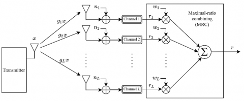
Figure 1. Block diagram of MRC system model
Let us consider an L-branch MRC receiver operating over i.n.i.d GG fading multipath channels. The received signal, $r_{i}$, at its ith antenna is expressed as [24]
$r_{i}=g_{i} x+n_{i},(i=1, \ldots, L)$ (39)
where, x is the complex transmitted symbol, with $\mathbb{E}\left[|x|^{2}\right]=E_{s}$ being the transmitted average symbol energy, $g_{i}=R_{i} e^{j \psi_{i}}(i=1, \ldots, L)$. where $R_{i}$ is the instantaneous fading amplitude corresponding to the received signals on the ith branch, assumed being i.n.i.d $G G\left(m_{i}, \beta_{i}, \Omega_{i}\right)$ distributed, $\psi_{i}$ is the corresponding instantaneous phase, while $n_{i}$ refers to the instantaneous additive white Gaussian noise (AWGN) with zero mean and single-sided power spectral density $N_{0}=\mathbb{E}\left[n_{i}^{2}\right]$, assumed to be identical for all branches. Moreover
$\Omega_{i}=m_{i}\left[\frac{\mathbb{E}\left[R_{i}^{2}\right]}{d_{2}\left(m_{i}, \beta_{i}\right)}\right]^{\frac{\beta_{i}}{2}}$ (40)
If each branch is weighted by $w_{i}$, then the linear combination of the received signals at the receiver's output, as shown in Figure 1, is expressed as
$r=\sum\limits_{i=1}^{L}{{{w}_{i}}}{{r}_{i}}=\sum\limits_{i=1}^{L}{{{w}_{i}}}{{g}_{i}}x+\sum\limits_{i=1}^{L}{{{w}_{i}}}{{n}_{i}}.$ (41)
Therefore, the output's SNR, $\gamma$, is given by
$\gamma =\frac{{{\left| \sum\limits_{i=1}^{L}{{{w}_{i}}}{{g}_{i}}x \right|}^{2}}}{\sum\limits_{i=1}^{L}{|{{w}_{i}}{{n}_{i}}{{|}^{2}}}}=\frac{{{E}_{s}}{{\left| \sum\limits_{i=1}^{L}{{{w}_{i}}}{{g}_{i}} \right|}^{2}}}{{{N}_{0}}\sum\limits_{i=1}^{L}{|{{w}_{i}}{{|}^{2}}}},$ (42)
By using Cauchy-Schwartz inequality in the numerator of (42), we obtain
$\gamma \le \frac{{{E}_{s}}\left( \sum\limits_{i=1}^{L}{|{{w}_{i}}{{|}^{2}}} \right)\left( \sum\limits_{i=1}^{L}{|{{g}_{i}}{{|}^{2}}} \right)}{{{N}_{0}}\sum\limits_{i=1}^{L}{|{{w}_{i}}{{|}^{2}}}},$ (43)
which is maximized if the weights $W_{i}$ are taken such that $w_{i}=g_{i}^{*}, \forall i \in\{1, \ldots, L\}$.
Thus, the resulting combiner SNR becomes
$\gamma =\sum\limits_{i=1}^{L}{\frac{{{E}_{s}}}{{{N}_{0}}}}|{{g}_{i}}{{|}^{2}}=\sum\limits_{i=1}^{L}{\frac{{{E}_{s}}}{{{N}_{0}}}}R_{i}^{2}=\sum\limits_{i=1}^{L}{{{\gamma }_{i}}},$ (44)
where the instantaneous SNR per symbol at the ith diversity channel is
${{\gamma }_{i}}=\frac{{{E}_{s}}}{{{N}_{0}}}R_{i}^{2}.$ (45)
Further, the average of $\gamma_{i}$ can be obtained from (45)
${{\bar{\gamma }}_{i}}=\frac{{{E}_{s}}}{{{N}_{0}}}\mathbb{E}[R_{i}^{2}]=\frac{{{E}_{s}}}{{{N}_{0}}}{{d}_{2}}({{m}_{i}},{{\beta }_{i}}){{\left( \frac{{{\Omega }_{i}}}{{{m}_{i}}} \right)}^{2/{{\beta }_{i}}}}.$ (46)
Note that if $R_{i}$ are i.i.d, then $\bar{\gamma}_{i}=\bar{\gamma}_{1}, \forall i$.
Furthermore, by using (2), the nth moment of $R_{i}$ can be expressed as
$\mu _{n}^{({{R}_{i}})}=\mathbb{E}\left[ R_{i}^{n} \right]={{d}_{n}}({{m}_{i}},{{\beta }_{i}}){{\left( \frac{{{\Omega }_{i}}}{{{m}_{i}}} \right)}^{n/{{\beta }_{i}}}}.$ (47)
4.2 Statistical analysis
In this Subsection, various metrics related to the performance of the considered WCS are derived.
4.2.1 Outage probability of the output SNR γ
Corollary 3. The outage probability, Pout, can be approximated as
${{P}_{out}}\approx a\lambda H_{2,2}^{1,1}\left[ \frac{{{\gamma }_{th}}}{\lambda }\left| \begin{matrix} \left( 1,1 \right);\left( b+1,1 \right) \\ \left( c+1,1 \right);\left( 0,1 \right) \\\end{matrix} \right. \right],$ (48)
where, γth denotes the minimum SNR threshold that guarantees the reliable communication and having the corresponding channel not in outage.
4.2.2 Moment of the output SNR $\gamma$
The nth moment of $\gamma$ is by definition $\mu_{n} \triangleq \mathbb{E}\left[\gamma^{n}\right]$. By applying (21), the nth moment of the MRC output SNR undergoing i.n.i.d GG fading channels can be approximated as
$\begin{align} & {{\mu }_{n}}={{\mathcal{M}}_{n+1}}\left[ {{f}_{\gamma }}(\gamma ) \right] \\ & =a{{\lambda }^{n+1}}\frac{\Gamma (c+n+1)}{\Gamma (b+n+1)}. \end{align}$ (49)
4.2.3 Average channel capacity
Proposition 2. Let $B_{w}$ be the channel bandwidth. The ACC under MRC diversity and i.n.i.d GG fading channels can be approximated as
$\bar{C}\approx \frac{a{{B}_{w}}}{\ln (2)}H_{3,3}^{3,1}\left[ \frac{1}{\lambda }\left| \begin{matrix} (-1,1);(0,1),(b,1) \\ (-1,1),(-1,1),(c,1);- \\\end{matrix} \right. \right].$ (50)
Proof: The ergodic capacity of the multipath channel under MRC diversity, per unit bandwidth, is given by [5]
$\begin{align} & \bar{C}={{B}_{w}}\mathbb{E}\left[ {{\log }_{2}}\left( 1+\gamma \right) \right] \\ & ={{B}_{w}}\int_{0}^{\infty }{{{\log }_{2}}}\left( 1+\gamma \right){{f}_{\gamma }}(\gamma )d\gamma . \end{align}$ (51)
The logarithmic function can be expressed as FHF [28]
$\ln \left( 1+\gamma \right)=H_{2,2}^{1,2}\left[ \gamma \left| \begin{matrix} (1,1),(1,1);- \\ (1,1);(0,1) \\\end{matrix} \right. \right].$ (52)
Then,
$\begin{align} & \bar{C}\approx \frac{a{{B}_{w}}}{2\pi jln(2)}\int_{\mathcal{C}}{\frac{\Gamma (c+s)}{\Gamma (b+s){{\lambda }^{-s}}}}\ \\ & \times \left( \int_{0}^{\infty }{{{\gamma }^{-s}}}H_{2,2}^{1,2}\left[ \gamma \left| \begin{matrix} (1,1),(1,1);- \\ (1,1);(0,1) \\\end{matrix} \right. \right]d\gamma \right)ds. \end{align}$ (53)
Now, using the Mellin transform (13) of FHF
$\begin{align} & \int_{0}^{\infty }{{{\gamma }^{-s}}}H_{2,2}^{1,2}\left[ \gamma \left| \begin{matrix} (1,1),(1,1);- \\ (1,1);(0,1) \\\end{matrix} \right. \right]d\gamma \\ & ={{\mathcal{M}}_{1-s}}\left( H_{2,2}^{1,2}\left[ \gamma \left| \begin{matrix} (1,1),(1,1);- \\ (1,1);(0,1) \\\end{matrix} \right. \right] \right) \\ & =\frac{\Gamma (2-s){{\Gamma }^{2}}(s-1)}{\Gamma (s)} \end{align}$ (54)
and substituting (54) into (53), (50) is attained, which concludes the proof of Proposition 2.
4.2.4 Average symbol error probability
Proposition 3. The ASEP for several coherent modulation techniques and MRC combiner operating under i.n.i.d GG multipath fading environment can be approximated by
${{\bar{P}}_{s}}(x)\approx \frac{\rho a}{\sqrt{\pi }\delta }\begin{array}{*{35}{l}} H_{3,2}^{1,2}\left[ \frac{1}{\delta \lambda }\left| \begin{matrix} (0,1),\left( -\frac{1}{2},1 \right);\left( b,1 \right) \\ \left( c,1 \right);(-1,1) \\\end{matrix} \right. \right] \\\end{array},$ (55)
where, $\varrho$ and $\delta$ are two parameters depending on the modulation scheme and summarized in Table 1 [29].
Table 1. Values of $\varrho$ et $\delta$ for some signaling constellations
|
Modulation |
M |
$\varrho$ |
$\delta$ |
|
BPSK |
2 |
1/2 |
1 |
|
BFSK |
2 |
1/2 |
1/2 |
|
M-PSK |
$\geq 4$ |
1 |
$\sin ^{2}(\pi / M)$ |
|
M-FSK |
$\geq 4$ |
$(M-1) / 2$ |
1/2 |
|
M-DPSK |
$\geq 2$ |
1 |
$2 \sin ^{2}(\pi / 2 M)$ |
|
M-QAM |
$\geq 4$ |
$2-2 / \sqrt{M}$ |
$1.5 /(M-1)$ |
|
M-PAM |
|
$(M-1) / M$ |
$3 /\left(M^{2}-1\right)$ |
Proof: The ASEP is evaluated as the expectation value of the instantaneous symbol error rate $P_{s}$ [5]
${{\bar{P}}_{s}}=\int_{0}^{\infty }{{{P}_{s}}}(\gamma ){{f}_{\gamma }}(\gamma )d\gamma ,$ (56)
where, $P_{s}$ is the conditional SER of various digital modulations, given by [29]
${{P}_{s}}(\gamma )\approx 2\varrho \text{Q}\left( \sqrt{2\delta \gamma } \right),$ (57)
with $Q(.)$ is the Gaussian Q-function defined as
$\text{Q}\left( x \right)=\frac{1}{\pi }\int_{0}^{\frac{\pi }{2}}{{{e}^{-\frac{{{x}^{2}}}{2{{\sin }^{2}}\phi }}}}d\phi ,x\ge 0$ (58)
Using an alternative Q-function representation (58), the conditional error probability (57) can be written as
${{P}_{s}}(\gamma )\approx \frac{2\rho }{\pi }\int_{0}^{\frac{\pi }{2}}{{{e}^{-\frac{\delta x}{{{\sin }^{2}}\phi }}}}d\phi ,\gamma \ge 0.$ (59)
By substituting (59) into (56), the ASEP can be expressed in terms of MGF as
$\begin{align} & {{{\bar{P}}}_{s}}\approx \frac{2\rho }{\pi }\int_{0}^{\infty }{\left\{ \int_{0}^{\frac{\pi }{2}}{{{e}^{-\frac{\delta x}{{{\sin }^{2}}\phi }}}}d\phi \right\}}{{f}_{\gamma }}(\gamma )d\gamma \\ & \approx \frac{2\rho }{\pi }\int_{0}^{\frac{\pi }{2}}{{{M}_{\gamma }}}\left( -\frac{\delta }{{{\sin }^{2}}\phi } \right)d\phi . \end{align}$ (60)
By rewriting the MGF given in (38) in terms of Gamma function, we get an approximate expression of ASEP as
$\begin{align} & {{{\bar{P}}}_{s}}\approx \frac{2\rho a}{\pi \delta }\frac{1}{2i\pi }\int\limits_{\mathcal{C}}{\frac{\Gamma \left( c+s \right)\Gamma \left( 1-s \right)}{\Gamma \left( b+s \right)}}{{\left( \frac{1}{\delta \lambda } \right)}^{-s}} \\ & \ \ \times \left\{ \int_{0}^{\frac{\pi }{2}}{{{\sin }^{2-2s}}}\left( \phi \right)d\phi \right\}ds, \end{align}$ (61)
where, $\int_{0}^{\frac{\pi}{2}} \sin ^{2-2 s}(\phi) d \phi$ can be expressed, when $\mathfrak{R}(s)<\frac{3}{2}$, in terms of Beta function [25] as
$\begin{align} & \int_{0}^{\frac{\pi }{2}}{{{\sin }^{2-2s}}}\left( \phi \right)d\phi =\frac{1}{2}B\left( \frac{3}{2}-s,\frac{1}{2} \right) \\ & =\frac{\sqrt{\pi }}{2}\frac{\Gamma \left( \frac{3}{2}-s \right)}{\Gamma \left( 2-s \right)}. \end{align}$ (62)
Finally, incorporating (62) into (61), (55) is attained, which concludes the proof of Proposition 3.
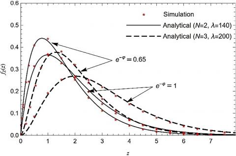
In this section, the FHF were evaluated using Mathematica software. All the analytical expressions derived are validated using MATLAB software via Monte-Carlo simulations, as shown in algorithm 1, by generating $10^{7} N$ generalized gamma distributed random numbers. Further, the inverse transform sampling method [30] is employed, along with the exponential decaying power delay profile with equispaced delays [31]:
$\mu_{1}^{\left(z_{i}\right)}=\mu_{1}^{\left(z_{1}\right)} e^{-\varphi(i-1)}, \forall i \in\{1, \ldots, N\}$ (63)
where, $\varphi$ stands for the average power decay factor.
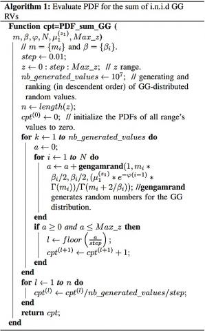
In Figure 2, the tightness of the proposed approximate PDF is obviously observed over the entire range of z for $e^{-\varphi}=\{1,0.9\}, m=2, \beta=3$, and different values of N (N= 10, 25, 50). One can see that the greater N is, the more curves shift to the right. This is because, the greater N is, the greater $\mu_{1}$ is, and consequently the maximum value of the probability is attained around such an average.
Figure 2. PDF of i.n.i.d GG sums for $m=2, \beta=3, \lambda=200$ and various values of N, and $\varphi$
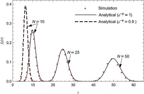
Figure 3. Approximated and simulated PDF of the sum of GG RVs for ( $m=1$ and $\beta=2$)
In Figure 3, the approximated and the simulated PDF of sum i.n.i.d GG RVs, Z, are plotted using (21) and via Monte-Carlo simulation with the help (21) of algorithm 1 over the z's range [0,8]. It can be observed that the proposed approximation is tight for all values of $\varphi$ and N, validating the accuracy of (21). Moreover, the greater $\varphi$ and N are, the greater $\mu_{1}$ is. On the other hand, according to (21) related to $\lambda$ term of theorem 1, and from the condition convergence (28), the value of $\lambda$ is chosen to be greater than the maximum value of $\Delta$ computed for $m=1, \beta=2$, and $\varphi=\{0,-\ln (0.65)\}$ (i.e., $\Delta=4.73$ for $N=2$ and $\Delta=6$ for $N=3$).
In Figure 4, the approximated PDF versus z, is plotted from (21) for $N=3, \varphi=\{0,-\ln (0.2)\}, m=\{2,4\}$, and $\beta=2$. The value of $\lambda=100$ should be chosen greater than the maximum value of $\Delta$computed for $m=2$, and $\varphi=-\ln (0.2)$ (i.e., 2.49). It is worth mentioning that the PDF becomes narrower and closer to 1 at $\mu_{1}=z$ with the increase of m.
Figure 5 shows both approximated and simulated CDF computed for $N=4, m=3, \beta=\{1,3\}, \lambda=200$, and $e^{-\varphi}=\{1,1.2\}$. It can be observed that the curves match well over the entire range. Moreover, the KS statistical test [32] measured for $N \leq 50, e^{-\varphi}=\{1,1.2\}, m=3, \beta=3$, $\lambda=200$, and a given significance level 0.05 shows that the goodness-of-fit calculated by averaging 15 results obtained for 300 samples remains less than the associated critical level 0.085714, for which the null hypothesis is not rejected, i.e., the approximate CDF in confirmity with the data got by simulation.
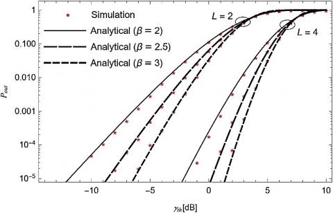
Figure 6 depicts both the approximate and simulated outage probability $P_{\text {out }}$ versus $\gamma_{t h}$ (in dB) for $m=2, \varphi=-\ln (1.2)$, and different values of $\gamma_{t h}$ and $\frac{\mu_{2}}{\mu_{1}}<15 \mathrm{~dB}$. The parameter $\lambda$ is chosen to be greater than the maximal value of $\gamma_{t h}$ to ensure convergence of OP since $\frac{\mu_{2}}{\mu_{1}}<15 \mathrm{~dB}$dB for the two cases $L=2$, and $L=4$. It is evident that the analytical result, evaluated using (48), are highly accurate with its simulation counterpart. Also, it can be seen that the decrease in OP can be achieved by increasing either L or $\beta$, for which the system becomes more reliable.
Figure 4. Analytical PDF of the sum of three GG RVs for $\beta=2$ and $\lambda=100$
Figure 5. CDF of i.n.i.d GG sums for $N=4$ and $m=3$
Figure 6. OP for L-branch receiver and m=2
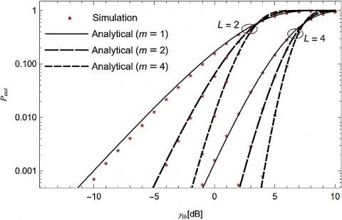
Figure 7 shows the evolution of OP versus minimum SNR threshold $\gamma_{t h}$ [dB], plotted from (48) for $\beta=2.5$, L-branch MRC combiner, and various values of m. Evidently, the greater both the diversity order L and the fading severity m are, the smaller OP is, leading to more reliable system.
Figure 7. OP vs minimum SNR for L-branch MRC receiver and $\beta=2.5$
Figure 8. Normalized ACC vs total average SNR at the output of L-branch MRC receiver for $m=1$ and $\lambda=400$
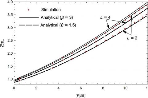
Figure 8 depicts both the analytical and the simulated normalized ACC as a function of average output SNR, $\bar{\gamma}$, for two- and four-branch MRC receiver, and $e^{-\varphi}=1.2$. The average SNR of signal at the first branch's input $\bar{\gamma}_{1}$ was chosen in $[-2.7 \mathrm{~dB}, 15.74 \mathrm{~dB}]$ and $[-6.57 \mathrm{~dB}, 11.87 \mathrm{~dB}]$ for L=2 and 4, respectively. The value of $\lambda$ should be greater than 86.98 to ensure the convergence of the HD given in (50). Clearly, the approximate analytical expression for ACC matches perfectly the simulated one for different settings of the system parameters. Also, the ACC is monotonically increasing with the increase of $\bar{\gamma}, \beta$, and L, leading to a more reliable system.
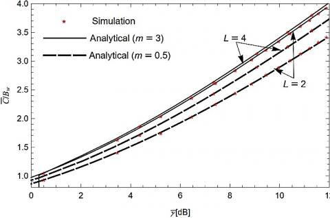
Figure 9 depicts both the analytical and the simulated normalized ACC as a function of average output SNR for two- and four-branch MRC receiver, and $e^{-\varphi}=1.2$. $\bar{\gamma}_{1}$ was chosen in $[-2.7 \mathrm{~dB}, 15.74 \mathrm{~dB}]$ and $[-6.57 \mathrm{~dB}, 11.87 \mathrm{~dB}]$ for L=2 and 4, respectively. The value of $\lambda$ should be greater than 90.56 to ensure the convergence of the HD given in (50). Obviously, the approximate analytical expression for ACC matches perfectly the simulated one for different settings of the system parameters. Besides, it is noteworthy that the ACC is monotonically increasing with the increase of $\bar{\gamma}, m$, and L, leading to a system quality improvement.
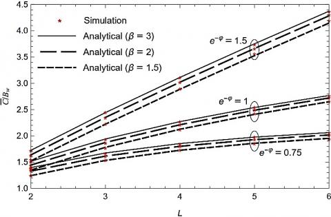
In Figure 10, both the approximate and simulated ACC per bandwidth versus L are plotted for m=1, and various values of $\beta$ and $\varphi$. The value of $\lambda$ should be greater than 37.03 computed for $L=6, e^{-\varphi}=1.5$, and $\beta=3$. It is clearly noticed that both curves are matching for various configuration settings. Also, the greater both the diversity m=1 order L and the fading severity $\beta$ are, the better ACC is.
Figure 9. Normalized ACC vs total average SNR at the output of L-branch MRC receiver for $\beta=2$ and $\lambda=400$
Figure 10. Normalized ACC vs L for m=1 and $\lambda=400$
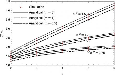
Figure 11. Normalized ACC vs L for $\beta=2$ and $\lambda=400$
Figure 11 illustrates both approximate and simulated ACC per bandwidth versus for $\beta=2$, and various values of m and $\varphi$. Again, both curves are perfectly matching, which proves the accuracy of our result.
Figure 12 plots the analytical expression and simulates ASEP versus the average SNR at the MRC output from (55) and (56), respectively, for $L=4, e^{-\varphi}=1.2$, and for different values of M, with the help of Table 1. One can notice that, the analytical results perfectly match the simulated ones. The branch average SNR $\bar{\gamma}_{1}$ varies between -12.7 dB and 20.3 dB. It is worthwhile to mention that the smaller M is, the smaller ASEP is. Also, ASEP decreases with the increase of $\bar{\gamma}$, leading to system quality enhancement.
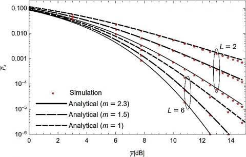
In Figure 13, the analytical ASEP $\bar{P}_{s}$ is plotted, from (55), as a function of $\bar{\gamma}$, for BDPSK modulation scheme, based on Table 1, $\beta=3$, and several values of m and L. Clearly, the ASEP reduces with the increase of $\bar{\gamma}$. Besides, the system performance improves with an increase of both the diversity order L and the fading severity m.
Figure 12. ASEP for M-PSK modulation scheme vs $\bar{\gamma}$ for $L=4, m=2, \beta=3$, and $\lambda=400$
Figure 13. ASEP for BDPSK modulation technique vs $\bar{\gamma}$ for $\beta=3, \varphi=0$, and two values of L
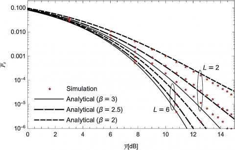
Figure 14. ASEP vs gamma^{bar} for BDPSK, m=2, $\varphi=0$, and two values of L
Figure 14, presents both the approximate and simulated ASEP $\bar{P}_{S}$ as a function of $\bar{\gamma}$, is plotted for BDPSK modulation, m=2, and several values of $\beta$, and L. Again, the greater both L and $\beta$ are, the smaller the ASEP is.
New accurate approximate expressions for the PDF, and CDF of i.n.i.d GG RVs sums were derived in this paper. The two proposed expressions have been validated by performing their simulation. A perfect match between the approximate expressions and simulate ones has been noticed. This approach is quite useful in the field of wireless communications where the sum of RVs' distribution is necessary for performance metrics evaluation purposes. Pointedly, accurate approximations for MRC receiver performance criteria experiencing GG fading channels such as OP, ACC, and ASEP have been derived. All derived analytical results are proved via Monte-Carlo simulations.
All analytical results show that the greater is the parameter $\lambda$ (appearing as a denominator in the first argument of the Fox’s H-function (21)), the higher is the evaluation time. Therefore, the only flaw in the proposed method that should be omitted exists in the lambda parameter, $\lambda$, and that it could be addressed adequately in the next paper.
The results obtained are limited only to i.n.i.d GG RVs. Based on the moment-based approximation method by estimating the first 5 moments of the sums of GG RVs instead of only three, the investigation may provide a potential direction for future work in correlated GG.
|
ACC |
average channel capacity |
|
ASEP |
average symbol error probability |
|
CDF |
commulative density function |
|
FHF |
Fox’s H-function |
|
GG |
generalized gamma |
|
HD |
H-distribution |
|
i.n.i.d |
independent and not necessarily identically distributed |
|
MGF |
moment-generating function |
|
MRC |
maximal-ratio combining |
|
OP |
outage probability |
|
|
probability density function |
|
RVs |
random variables |
|
SNR |
signal-to-noise ratio |
|
WCSs |
wireless communication systems |
|
Notations |
|
|
$\Gamma(.)$ |
Euler Gamma function [25, eq. (6.1.1)] |
|
$\mathbb{E}[.]$ |
Expectation operator |
|
$\mu_{r}$ |
rth moment |
|
$\mathbb{V}[.]$ |
Variance function |
|
$Q(.)$ |
Gaussian Q-function [25, eq. (26.2.3)] |
|
$H[.]$ |
Fox’s H-function [12, eq. (6.2.1)] |
|
$\mathcal{C}$ |
Infinite contour integral in the complex plane |
|
$\mathcal{H}(.)$ |
Integrand of Mellin-Barnes integral of $H[.]$ |
|
$\mathcal{M}_{s}\{.\}$ |
Mellin transform of $H[.]$ [12, eq. (2.8.9)] |
|
$\mathcal{M}_{z}^{-1}\{\cdot\}$ |
Inverse Mellin transform [12, eq. (2.8.10)] |
|
$\mathbb{R}^{+}$ |
Set of non-negative real numbers $[0, \infty)$ |
|
$f_{Z}(.)$ |
Probability density function of GG RV Z |
|
$F_{Z}(.)$ |
Cumulative density function of GG RV Z |
|
$Z \sim G G(.,., .)$ |
Z is GG distributed |
|
$\bar{P}_{s}$ |
Average symbol error probability |
[1] Fox, C. (1961). The G and H functions as symmetrical Fourier kernels. Transactions of the American Mathematical Society, 98(3): 395-429. https://doi.org/10.2307/1993339
[2] Saxena, R.K., Saxena, R., Kalla, S.L. (2010). Computational solution of a fractional generalization of the Schrödinger equation occurring in quantum mechanics. Applied Mathematics and Computation, 216(5): 1412-1417. https://doi.org/10.1016/j.amc.2010.02.041
[3] Mathai, A.M., Saxena, R.K., Haubold, H.J. (2009). The H-function: Theory and applications. Springer Science & Business Media.
[4] Yilmaz, F., Alouini, M.S. (2012). A novel unified expression for the capacity and bit error probability of wireless communication systems over generalized fading channels. IEEE Trans. Commun., 60: 1862-1876. https://doi.org/10.1109/TCOMM.2012.062512.110846
[5] Simon, M.K., Alouini, M.S. (2005). Digital Communication over Fading Channels. John Wiley & Sons.
[6] Coulson, A.J., Williamson, A.G., Vaughan, R.G. (1998). Improved fading distribution for mobile radio. IEE Proceedings-Communications, 145(3): 197-202. https://doi.org/10.1049/ip-com:19981991
[7] Griffiths, J., McGeehan, J.P. (1982). Interrelationship between some statistical distributions used in radio-wave propagation. In IEE Proceedings F-Communications, Radar and Signal Processing, 129(6): 411-417. https://doi.org/10.1049/ip-f-1.1982.0063
[8] Stacy, E.W. (1962). A generalization of the Gamma distribution. The Ann. Math. Statist., 33(3): 1187-1192. https://doi.org/10.1214/aoms/1177704481
[9] El Bouanani, F., da Costa, D.B. (2018). Accurate closed-form approximations for the sum of correlated Weibull random variables. IEEE Wireless Communications Letters, 7(4): 498-501. https://doi.org/10.1109/LWC.2017.2789280
[10] El Bouanani, F., Ben-Azza, H. (2017). Unified analysis of EGC diversity over Weibull fading channels. International Journal of Communication Systems, 30(1): e2925. https://doi.org/10.1002/dac.2925
[11] El Bouanani, F. (2014). A new closed-form approximation for MRC receiver over non-identical Weibull fading channels. In Proc. International Wireless Communications and Mobile Computing Conference (IWCMC), pp. 600-605. https://doi.org/10.1109/IWCMC.2014.6906424
[12] Springer, M.D. (1979). The Algebra of Random Variables. Wiley, New York.
[13] Bodenschatz, C.D. (1992). Finding an H-function distribution for the sum of independent H-function variates. Air Force Inst of Tech Wright-Patterson AFB OH.
[14] Jacobs, H., Barnes, J.W., Cook, I.D. (1987). Applications of the h-function distribution in classifying and fitting classical probability distributions. American Journal of Mathematical and Management Sciences, 7: 131-147. https://doi.org/10.1080/01966324.1987.10737211
[15] Cook Jr, I.D. (1981). The H-function and probability density functions of certain algebraic combinations of independent random variables with H-function probability distribution. Air Force Inst of Tech Wright-Patterson AFB OH.
[16] Aalo, V.A., Efthymoglou, G.P., Piboongungon, T. Iskander, C.D. (2007). Performance of diversity receivers in generalised Gamma fading channels. IET Commun., 1(3): 341-347. https://doi.org/10.1049/iet-com:20050235
[17] Sagias, N.C., Mathiopoulos, P.T. (2005). Switch diversity receivers over generalized Gamma fading channels. IEEE Commun. Lett., 9(10): 871-873. https://doi.org/10.1109/LCOMM.2005.10026
[18] Di Renzo, M., Graziosi, F., Santucci, F. (2010). Channel capacity over generalized fading channels: A novel MGF-based approach for performance analysis and design of wireless communication systems. IEEE Transactions on Vehicular Technology, 59(1): 127-149. https://doi.org/10.1109/TVT.2009.2030894
[19] Bithas, P.S., Sagias, N.C., Tsiftsis, T.A. (2008). Performance analysis of dual-diversity receivers over correlated generalised Gamma fading channels. IET Communications, 2(1): 174-178. https://doi.org/10.1049/iet-com:20070207
[20] Aalo, V.A., Piboongungon, T., Iskander, C.D. (2005). Bit-Error rate of binary digital modulation schemes in generalized gamma fading channels. IEEE Commun. Lett., 9(2): 139-141. https://doi.org/10.1109/LCOMM.2005.02027
[21] Cheng, J., Berger, T. (2003). Performance analysis for MRC and postdetection EGC over generalized gamma fading channels. In Proc. IEEE wireless communications and networking conference (WCNC’03), pp. 120-125. http://ir.lib.nthu.edu.tw/handle/987654321/58122
[22] Chauhan, P.S., Rana, V., Kumar, S., Soni, S.K., Pant, D. (2019). Performance analysis of wireless communication system over nonidentical cascaded generalised gamma fading channels. Int. J. Commun. Syst., 32: 1-15. https://doi.org/10.1002/dac.4004
[23] Sagias, N.C., Mathiopoulos, P.T., Bithas, P.S., Karagiannidis, G.K. (2005). On the distribution of the sum of generalized gamma variates and applications to satellite digital communications. In Proc. 2nd International Symposium on Wireless Communication Systems, pp. 785-789. https://doi.org/10.1109/ISWCS.2005.1547816
[24] Sagias, N.C., Karagiannidis, G.K., Mathiopoulos, P.T., Tsiftsis, T.A. (2006). On the performance analysis of equal-gain diversity receivers over generalized gamma fading channels. IEEE Transactions on Wireless Communications, 5(10): 2967-2975. https://doi.org/10.1109/TWC.2006.05301
[25] Stacy, E.W., Mihram, G.A. (1965). Parameter estimation for a generalized gamma distribution. Technometrics, 7(3): 349-358. https://doi.org/10.2307/1266594
[26] Dadpaya, A., Soofi, E. S., Soyer, R. (1965). Information measures for generalized gamma family. Journal of Econometrics, 138(2): 568-585. https://doi.org/10.1016/j.jeconom.2006.05.010
[27] Abramowitz, M., Stegun, I.A. (1964). Handbook of mathematical functions with formula graphs and mathematical tables. National Bureau of Standards, Applied Mathematical Series, 55: 319. https://doi.org/10.1119/1.15378
[28] Prudnikov, A.P., Brychkov, Y.A., Marichev, O.I. (1990). Integrals and series, more special functions. Gordon and Breach Science. New York. https://doi.org/10.2307/2007975
[29] Goldsmith, A. (2005). Wireless Communications. Cambridge University Press. ISBN: 0521837162
[30] Taqdees, S.W. (2020). Gengamrand(n,Alpha, Beta, a) (https://www.mathworks.com/matlabcentral/fileexchange/48220-gengamrand-n-alpha-beta-a), MATLAB Central File Exchange.
[31] Kong, N., Milstein, L.B. (2000). SNR of generalized diversity selection combining with nonidentical Rayleigh fading statistics. IEEE Transactions on Communications, 48: 1266-1271. https://doi.org/10.1109/26.864164
[32] Frank, J., Massey, Jr. (1951). The Kolmogorov-Smirnov Test for Goodness of Fit. Journal of the American Statistical Association, 46(253): 68-78. https://doi.org/10.1080/01621459.1951.10500769