Sachidananda Sahoo | Kishore Kumar Prusty | Satyaranjan Mishra*
© 2021 IIETA. This article is published by IIETA and is licensed under the CC BY 4.0 license (http://creativecommons.org/licenses/by/4.0/).
OPEN ACCESS
The present study reveals the heat and mass transfer on the MHD flow of micropolar fluid in a porous medium within a rotating frame. In order to facilitate osillatory plate velocity with constant suction and first order chemical reaction has been considered. Using small perturbation approximation, the governing non-dimensional equations are solved. The influence of pertinent physical quantities on the flow phenomena have been presented graphically. The skin friction coefficient, wall couple stress, Nusselt and Sherwood number have also computed for different flow parameters and have presented in table. In the study, the applied magnetic field sets in to produce the resistive force i.e. the Lorentz force that resists the fluid motion throughout the domain. Attenuation in the Prandtl number is because of the slower thermal diffusivity resulted in a sharp reduction in the thermal boundary layer thickness. The retardation in the polar fluid concentration is greater in amount for the influence of heavier species.
MHD flow, micropolar fluid, rotating frame, chemical reaction, porous medium
In comparison to Newtonian fluids, non-Newtonian fluids have several interesting applications in various areas due to the physics of the problems. From these fluids microploar fluid is became popular in the mind of young researchers for their varied applications in industries as well as in engineering. Though the movement of the fluid particles is randomly oriented and there is a translation as well as rotation occurs in each volume element of the fluid, it revealed several interesting phenomena. Eringen [1, 2] originated the theoretical concept of micropolar fluids and thermo micropolar fluids for the characteristics in particular animal blood, exotic lubricants, polymeric fluids, liquid crystals, etc. due to microrotation, these fluids exhibit microscopic effects arising from local structure of the fluid particles. Ariman et al. [3, 4] provides excellent reviews about the mechanics of the micropolar fluid.
The exploration of heat transport phenomena is vital in the case of moving fluid with incorporating the study of both exothermic and endothermic chemical reaction. Flow over a stretching surface for the interaction of chemical reaction that takes due to the combine effects of working fluid and the foreign mass in the various chemical engineering processes. Depending upon the several physical properties its order varies. In general, reaction rate is related to the species concentration is known as first-order reaction, one of the simplest and widely used chemical reactions. Time-dependent flow of polar fluid in a rotating frame of reference with the chemical reaction and heat source was organized by Bakr [5]. He has proposed his investigation by considering oscillatory plate velocity in conjunction with constant suction. Further, flow past an oscillatory vertical plate for a micropolar fluid with the Newtonian heating boundary conditions is worked out by Hussanan et al. [6]. Sheri and Shamshuddin [7] have analyzed the influence of dissipative heat transport phenomena of MHD polar fluid in conjunction with reactive agents. Rout et al. [8] have studied the behavior of magnetic parameter applied in the normal direction for the flow of a conducting micropolar fluid. The proposed boundary value problem is conducted over the plate placed vertically where the wall temperature and concentration varies with time. In viewing to the importance of aforesaid discussion, Animasaun [9] has analyzed the flow of micropolar fluid with the inclusion of temperature dependent viscosity and thermal conductivity. The crux of their investigation is the study of melting boundary condition.
Mahmoud [10] has proposed the flow of a non-Newtonian fluid past an extended surface embedding with porous matrix. In addition, an enhanced flow characteristic is analyzed by incorporating the surface slip, and variable viscosity for the behavior of reactive agents. In a recent study, Khan [11] has used a non-Darcy Jeffry model using modified Darcy’s law. In his investigation the proposed model is based on fractional calculus for the non-Newtonian fluid. Dessie and Kishan [12] have studied the influenced heat characteristics incorporating viscous dissipation in a MHD boundary layer flow past an extended surface. In their work, they have proposed the effects of variable viscosity in conjunction with external heat source/sink. Mishra et al. [13] have carried out the flow of a conducting viscoelastic fluid for the behavior of chemical reaction. Further, Mishra and his co-workers [14-16] have worked out several studies on the flow properties of various non-Newtonian fluid for several physical parameters with different geometries.
From various applications, the crude oil extraction is one in which the role of porosity plays a vital role. In addition, ground water hydrology, geothermal systems, packed bed, etc. are the example of different processes for those the medium is filled with porous materials. It is the measure of the empty spaces in the material and in a total volume; it is the fraction of empty volume. In a flow channel it varies from location to location depending upon the pattern. It can be used in various fields i.e. metallurgy, materials, manufacturing, mechanics and engineering etc. To the best of author’s knowledge, the flow of MHD micropolar fluid with heat and mass transfer in a rotating frame of reference in presence of porous medium has not been addressed so far. Therefore, we have extended the work of Bakr [5] by considering the flow in a porous medium. So, our study is now confined to heat transport mechanism of a conducting polar fluid within a rotating frame embedding with porous medium.
Natural convection of a three-dimensional time-dependent flow of micropolar fluid over a semi-infinite vertical moving porous plate in a porous medium is presented in this study. The magnetic field applied in the direction transverse with uniform heat source also assumed in the said discussion. It is assumed that the plate velocity u*(t) oscillatory and defined by u*(t*) = Ur(1 + $\varepsilon$cos nt) where time, t and frequency, n*. The direction of the flow along the x*-axis, towards the direction (upward direction) of the plate and z*-axis is normal to it. Initially, both the fluid and the plate are in rest and as time varies i.e. t* > 0, the system is allowed to rotate within a rotating frame $\Omega$ about the z*-axis. Magnetic field of uniform strength B0 is applied along the z* direction (Figure 1).
The conservation of electric charge proposed by $\nabla$· J = 0 implises Jz = constant, where J= (Jx, Jy, Jz). Here, Jz = 0, since the plate is electrically non-conducting. Depending upon the physical significance of the geometry all physical quantities depend on z* and t* only.
Figure 1. Flow geometry
The governing equations of the problem are
$\frac{\partial w^{*}}{\partial z^{*}}=0$ (1)
$\begin{aligned} \frac{\partial u^{*}}{\partial t^{*}}+w^{*} \frac{\partial u^{*}}{\partial z^{*}} &-2 \Omega v^{*}=\left(v+\frac{\alpha}{\rho}\right) \frac{\partial^{2} u^{*}}{\partial z^{* 2}}+g \beta\left(T-T_{\infty}\right) \\ &+g \hat{\beta}\left(C-C_{\infty}\right)-\sigma \frac{B_{0}^{2}}{\rho} u^{*}-\frac{v}{K} u^{*}-\frac{\alpha}{\rho} \frac{\partial n_{2}^{*}}{\partial z^{*}} \end{aligned}$ (2)
$\begin{aligned} \frac{\partial v^{*}}{\partial t^{*}}+w^{*} \frac{\partial v^{*}}{\partial z^{*}} &+2 \Omega u^{*}=\left(v+\frac{\alpha}{\rho}\right) \frac{\partial^2 v^{*}}{\partial z^{* 2}} \\ &-\sigma \frac{\beta_{0}^{2}}{\rho} v^{*}-\frac{v}{K} u^{*}+\frac{\alpha}{\rho} \frac{\partial n_{1}^{*}}{\partial z^{*}} \end{aligned}$ (3)
$\frac{\partial n_{1}^{*}}{\partial t^{*}}+w^{*} \frac{\partial n_{1}^{*}}{\partial z^{*}}=\frac{\gamma}{\rho \lambda^{*}} \frac{\partial^{2} n_{1}^{*}}{\partial z^{* 2}}$ (4)
$\frac{\partial {{n}_{2}}^{*}}{\partial {{t}^{*}}}+{{w}^{*}}\frac{\partial {{n}_{2}}^{*}}{\partial {{z}^{*}}}=\frac{\gamma }{\rho {{\lambda }^{*}}}\frac{{{\partial }^{2}}{{n}_{2}}^{*}}{\partial {{z}^{*}}^{2}}$ (5)
$\frac{\partial T}{\partial {{t}^{*}}}+{{w}^{*}}\frac{\partial T}{\partial {{z}^{*}}}=\frac{k}{\rho {{C}_{p}}}\frac{{{\partial }^{2}}T}{\partial {{z}^{*}}^{2}}-\frac{{{Q}_{H}}}{\rho {{C}_{p}}}(T-{{T}_{\infty }})$ (6)
$\frac{\partial C}{\partial {{t}^{*}}}+{{w}^{*}}\frac{\partial C}{\partial {{z}^{*}}}=D\frac{{{\partial }^{2}}C}{\partial {{z}^{*}}^{2}}-{{K}_{l}}(C-{{C}_{\infty }})$ (7)
The initial and boundary conditions of the model are
${{u}^{*}}=0\,,\,{{v}^{*}}=0\,,\,n_{1}^{*}=0\,,\,n_{2}^{*}=0\,,\,T=0\,,\,C={{C}_{\infty }}$ for ${{t}^{*}}\le 0$ (8)
$\left. \begin{align} & {{u}^{*}}={{U}_{r}}(1+\frac{\varepsilon }{2})({{e}^{i{{n}^{*}}{{t}^{*}}}}+{{e}^{-i{{n}^{*}}{{t}^{*}}}}),\,\,{{v}^{*}}=0, \\ & {{n}_{1}}^{*}=\frac{-1}{2}\frac{\partial {{v}^{*}}}{\partial {{z}^{*}}},\,{{n}_{2}}^{*}=\frac{1}{2}\frac{\partial {{u}^{*}}}{\partial {{z}^{*}}},\,T={{T}_{w}}\,,\,C={{C}_{w}}\,at\,{{z}^{*}}=0 \\ & {{u}^{*}}=0,{{v}^{*}}=0,\,n_{1}^{*}=0,\,n_{2}^{*}=0,\,T=0,\,C={{C}_{\infty }}\,\,as\,\,{{z}^{*}}\to \infty \\\end{align} \right\}$ (9)
for ${{t}^{*}}>0$, where $\varepsilon $ is a small constant quantity. According to the suggestion proposed by Ganapathy [17], we have assumed the oscillatory plate velocity which is given in Eq. (9).
We have now considered
${{w}^{*}}=-{{w}_{0}}$ (10)
Which satisfy Eq. (1) with unvarying w0 indicates the standard velocity at the plate and denotes suction/injection depending upon the sign. Following non-dimensional quantities are assumed for the transformation of the governing equations.
$\begin{align} & z=\frac{{{z}^{*}}U{}_{r}}{\upsilon }\,,\,u=\frac{{{u}^{*}}}{{{U}_{r}}},\,v=\frac{{{v}^{*}}}{{{U}_{r}}},\,t=\frac{{{t}^{*}}U_{r}^{2}}{\nu },n=\frac{{{n}^{*}}\upsilon }{U_{r}^{2}},\delta =\frac{\alpha }{\rho \upsilon }, \\ & {{n}_{1}}=\frac{\upsilon }{U_{r}^{2}}n_{1}^{*},{{n}_{2}}=\frac{\upsilon }{U_{r}^{2}}n_{2}^{*},\,\,\theta =\frac{T-{{T}_{\infty }}}{{{T}_{w}}-{{T}_{\infty }}},\,\,{{K}_{p}}=\frac{K{{U}_{r}}^{2}}{{{\upsilon }^{2}}},R=\frac{2\Omega \upsilon }{U_{r}^{2}}, \\ & \,\,\phi =\frac{C-{{C}_{\infty }}}{{{C}_{w}}-{{C}_{\infty }}},\,\,Sc=\frac{\upsilon }{D},Pr=\frac{\mu {{C}_{p}}}{k},Gr=\frac{g\beta \upsilon ({{T}_{w}}-{{T}_{\infty }})}{U_{r}^{3}},\, \\ & s=\frac{{{w}_{o}}}{{{U}_{r}}},Gm=\frac{g\hat{\beta }\upsilon ({{C}_{w}}-{{C}_{\infty }})}{U_{r}^{3}},S=\frac{{{Q}_{H}}{{\upsilon }^{2}}}{U_{r}^{2}k},Kc=\frac{{{K}_{l}}\upsilon }{{{U}_{r}}},\,\, \\ & M=\frac{\sigma B_{0}^{2}\upsilon }{\rho U_{r}^{2}},\,\lambda =\frac{Kc}{u{{\lambda }^{*}}}=(1+\frac{1}{2}\delta ), \\\end{align}$
Imposing above quantities and Eq. (10) the non-dimensional form of the governing equations is,
$\begin{align} & \frac{\partial u}{\partial t}-s\frac{\partial u}{\partial z}-Rv=(1+\delta )\frac{{{\partial }^{2}}u}{\partial {{z}^{2}}}+ \\ & \,\,\,\,\,\,\,\,\,\,\,\,\,\,\,Gr\theta +Gm\phi -(M+\frac{1}{Kp})u-\delta \frac{\partial {{n}_{2}}}{\partial z} \\\end{align}$ (11)
$\frac{\partial v}{\partial t}-s\frac{\partial v}{\partial z}+Ru=(1+\delta )\frac{{{\partial }^{2}}v}{\partial {{z}^{2}}}-(M+\frac{1}{Kp})v-\delta \frac{\partial {{n}_{1}}}{\partial z}$ (12)
$\frac{\partial {{n}_{1}}}{\partial t}-s\frac{\partial {{n}_{1}}}{\partial z}=\lambda \frac{{{\partial }^{2}}{{n}_{1}}}{\partial {{z}^{2}}}$ (13)
$\frac{\partial {{n}_{2}}}{\partial t}-s\frac{\partial {{n}_{2}}}{\partial z}=\lambda \frac{{{\partial }^{2}}{{n}_{2}}}{\partial {{z}^{2}}}$ (14)
$\frac{\partial \theta }{\partial t}-s\frac{\partial \theta }{\partial z}=\frac{1}{Pr}\frac{{{\partial }^{2}}\theta }{\partial {{z}^{2}}}-\frac{S}{Pr}\theta $ (15)
$\frac{\partial \phi }{\partial t}-s\frac{\partial \phi }{\partial z}=\frac{1}{Sc}\frac{{{\partial }^{2}}\phi }{\partial {{z}^{2}}}-Kc\phi $ (16)
The corresponding initial and boundary conditions in non-dimensional form are
$u=0,v=0,{{n}_{1}}=0,{{n}_{2}}=0,\theta =0,\phi =0\,\,for\,\,t\le 0$ (17)
$\left. \begin{align} & u=1+\frac{\varepsilon }{2}({{e}^{int}}+{{e}^{-int}}),v=0,{{n}_{1}}=-\frac{1}{2}\frac{\partial v}{\partial z}, \\ & {{n}_{2}}=\frac{1}{2}\frac{\partial u}{\partial z},\theta =1,\phi =1\,\,at\,\,z=0 \\ & u=v={{n}_{1}}={{n}_{2}}=\theta =\phi =0\,\,as\,\,z\to \infty \\\end{align} \right\}\,\,\,for\,t>0$ (18)
To solve the equations (11)-(16), we have considered
$U=u+iv\,\,,\,\,N={{n}_{1}}+i{{n}_{2}}$ (19)
Now with the help of Eq. (19), Eqns. (11)-(16) are reduced to
$\begin{align} & \frac{\partial U}{\partial t}-s\frac{\partial U}{\partial z}+iRU=(1+\delta )\frac{{{\partial }^{2}}U}{\partial {{z}^{2}}}+ \\ & \,\,\,\,\,\,\,\,\,\,\,Gr\theta +Gm\phi -\left( M+\frac{1}{Kp} \right)U+i\delta \frac{\partial N}{\partial z} \\\end{align}$, (20)
$\frac{\partial N}{\partial t}-s\frac{\partial N}{\partial z}=\lambda \frac{{{\partial }^{2}}N}{\partial {{z}^{2}}}$, (21)
$\frac{\partial \theta }{\partial t}-s\frac{\partial \theta }{\partial z}=\frac{1}{Pr}\frac{{{\partial }^{2}}\theta }{\partial {{z}^{2}}}-\frac{S}{Pr}\theta $, (22)
$\frac{\partial \phi }{\partial t}-s\frac{\partial \phi }{\partial z}=\frac{1}{Sc}\frac{{{\partial }^{2}}\phi }{\partial {{z}^{2}}}-Kc\phi $, (23)
The associated boundary conditions are
$U=0,N=0,\theta =0,\phi =0\,\,\,for\,\,t\le 0$, (24)
$\left. \begin{align} & U=1+\frac{\varepsilon }{2}({{e}^{int}}+{{e}^{-int}}),N=\frac{i}{2}\frac{\partial U}{\partial z},\theta =1,\phi =1\,\,at\,\,z=0 \\ & U=N=\theta =\phi =0\,\,\,as\,\,z\to \infty \\\end{align} \right\}\,\,for\,\,t>0$ (25)
In order to solve Eqns. (20)-(23) satisfying Eq. (25), we have defined the followings according to Ganapathy [17].
$U(z,t)={{U}_{0}}(z)+\frac{\varepsilon }{2}\left( {{e}^{int}}{{U}_{1}}(z)+{{e}^{-int}}{{U}_{2}}(z) \right)$ (26)
$N(z,t)={{N}_{0}}(z)+\frac{\varepsilon }{2}\left( {{e}^{int}}{{N}_{1}}(z)+{{e}^{-int}}{{N}_{2}}(z) \right)$ (27)
$\theta (z,t)={{\theta }_{0}}(z)+\frac{\varepsilon }{2}\left( {{e}^{int}}{{\theta }_{1}}(z)+{{e}^{-int}}{{\theta }_{2}}(z) \right)$ (28)
$\phi (z,t)={{\phi }_{\,0}}(z)+\frac{\varepsilon }{2}\left( {{e}^{int}}{{\phi }_{\,1}}(z)+{{e}^{-int}}{{\phi }_{\,2}}(z) \right)$ (29)
Substituting Eqns. (26)-(29) in Eqns. (20)-(23) and equating the coefficients of the harmonic and non-harmonic terms and neglecting the terms of $\varepsilon^{2}$, we have the following set of equations.
$\begin{align} & (1+\delta ){{U}_{0}}^{\prime \prime }+s{{U}_{0}}^{\prime }-\left( M+\frac{1}{Kp}+iR \right){{U}_{0}} \\ & \,\,\,\,\,\,\,\,\,\,\,\,\,\,\,\,\,\,\,\,+Gr{{\theta }_{0}}+Gm{{\phi }_{0}}+i\delta {{N}_{0}}^{\prime }=0 \\\end{align}$ (30)
$\lambda {{N}_{0}}^{\prime \prime }+s{{N}_{0}}^{\prime }=0$ (31)
${{\theta }_{0}}^{\prime \prime }+sPr{{\theta }_{0}}^{\prime }-S{{\theta }_{0}}=0$ (32)
${{\phi }_{\,0}}^{\prime \prime }+sSc{{\phi }_{\,0}}^{\prime }-\lambda Sc{{\phi }_{\,0}}=0$ (33)
$\begin{align} & (1+\delta ){{U}_{1}}^{\prime \prime }+s{{U}_{1}}^{\prime }-\left( M+\frac{1}{Kp}+i(R+n) \right){{U}_{1}} \\ & \,\,\,\,\,\,\,\,\,\,\,\,\,\,\,\,\,\,\,\,\,\,\,\,\,\,\,\,\,\,\,\,\,\,\,+Gr{{\theta }_{1}}+Gm{{\phi }_{1}}+i\delta {{N}_{1}}^{\prime }=0 \\\end{align}$ (34)
$\lambda {{N}_{1}}^{\prime \prime }+s{{N}_{1}}^{\prime }-in{{N}_{1}}=0$ (35)
${{\theta }_{1}}^{\prime \prime }+sPr{{\theta }_{1}}^{\prime }-(S+inPr){{\theta }_{1}}=0$ (36)
${{\phi }_{1}}^{\prime \prime }+sSc{{\phi }_{1}}^{\prime }-(in+\lambda )Sc{{\phi }_{1}}=0$ (37)
$\begin{align} & (1+\delta ){{U}_{2}}^{\prime \prime }+s{{U}_{2}}^{\prime }-\left( M+\frac{1}{Kp}+i(R-n) \right){{U}_{2}} \\ & \,\,\,\,\,\,\,\,\,\,\,\,\,\,\,\,\,\,\,\,\,\,\,\,\,\,\,\,\,\,\,\,+Gr{{\theta }_{2}}+Gm{{\phi }_{\,2}}+i\delta {{N}_{2}}^{\prime }=0 \\\end{align}$ (38)
$\lambda {{N}_{2}}^{\prime \prime }+s{{N}_{2}}^{\prime }+in{{N}_{2}}=0$ (39)
${{\theta }_{2}}^{\prime \prime }+sPr{{\theta }_{2}}^{\prime }-(S-inPr){{\theta }_{2}}=0$ (40)
${{\phi }_{\,2}}^{\prime \prime }+sSc{{\phi }_{\,2}}^{\prime }+(in-\lambda )Sc{{\phi }_{2}}=0$ (41)
where the primes denote differentiation with respect to z.
The associated boundary conditions are
$\left. \begin{align} & {{U}_{0}}=1,{{N}_{0}}=\frac{i}{2}{{U}_{0}}^{\prime },{{\theta }_{0}}=1,{{\phi }_{\,0}}=1\,\,at\,\,z=0 \\ & {{U}_{0}}=0,{{N}_{0}}=0,{{\theta }_{0}}=0,{{\phi }_{\,0}}=0\,\,at\,\,z\to \infty \\\end{align} \right\}$ (42)
$\left. \begin{align} & {{U}_{1}}=1,{{N}_{1}}=\frac{i}{2}{{U}_{1}}^{\prime },{{\theta }_{1}}=0,{{\phi }_{\,1}}=0\,\,at\,\,z=0 \\ & {{U}_{1}}=0,{{N}_{1}}=0,{{\theta }_{1}}=0,{{\phi }_{\,1}}=0\,\,as\,\,z\to \infty \\\end{align} \right\}$ (43)
$\left. \begin{align} & {{U}_{2}}=1,{{N}_{2}}=\frac{i}{2}{{U}_{2}}^{\prime },{{\theta }_{2}}=0,{{\phi }_{\,2}}=0\,\,at\,\,z=0 \\ & {{U}_{2}}=0,{{N}_{2}}=0,{{\theta }_{2}}=0,{{\phi }_{\,2}}=0\,\,as\,\,z\to \infty \\\end{align} \right\}$ (44)
The solutions of the Eqns. (30)-(41) satisfying the conditions given in Eqns. (42)-(44) are given by
$\begin{align} & U={{A}_{1}}{{e}^{-{{m}_{1}}z}}+{{A}_{2}}{{e}^{-{{m}_{2}}z}}+{{A}_{3}}{{e}^{-{{m}_{3}}z}}+{{h}_{3}}{{e}^{-(s/\lambda )z}} \\ & \,\,\,\,\,\,\,\,\,+\frac{\varepsilon }{2}\left( ({{A}_{4}}{{e}^{-{{m}_{5}}z}}+{{h}_{6}}{{e}^{-{{m}_{4}}z}}){{e}^{int}} \right. \\ & \left. \,\,\,\,\,\,\,\,\,+({{A}_{5}}{{e}^{-{{m}_{7}}z}}+{{h}_{9}}{{e}^{-{{m}_{6}}z}}){{e}^{-int}} \right), \\\end{align}$ (45)
$N={{h}_{2}}{{e}^{-(s/\lambda )z}}+\frac{\varepsilon }{2}\left( {{h}_{5}}{{e}^{int-{{m}_{4}}z}}+{{h}_{8}}{{e}^{-(int+{{m}_{6}}z)}} \right)$ (46)
$\theta ={{e}^{-{{m}_{2}}z}}$ (47)
$\phi ={{e}^{-{{m}_{1}}z}}$ (48)
Furthermore, the shear stress at the plate may be written as
$\tau _{wx}^{*}={{\left[ (\mu +\alpha )\frac{\partial {{u}^{*}}}{\partial {{z}^{*}}}+\alpha n_{1}^{*} \right]}_{{{z}^{*}}=0}}=\rho U_{r}^{2}{{\left[ \left( 1+\delta \right)\frac{\partial u}{\partial z}-\frac{\delta }{2}\frac{\partial v}{\partial z} \right]}_{z=0}}$ ,
$\tau _{wy}^{*}={{\left[ (\mu +\alpha )\frac{\partial {{v}^{*}}}{\partial {{z}^{*}}}+\alpha n_{2}^{*} \right]}_{{{z}^{*}}=0}}=\rho U_{r}^{2}{{\left[ \left( 1+\delta \right)\frac{\partial v}{\partial z}+\frac{\delta }{2}\frac{\partial u}{\partial z} \right]}_{z=0}}$ ,
$\begin{align} & \tau _{w}^{*}=\tau _{wx}^{*}+i\tau _{wy}^{*}=\rho U_{r}^{2}{{\left[ (1+\delta )\frac{\partial U}{\partial z}+\frac{i\delta }{2}\frac{\partial U}{\partial z} \right]}_{z=0}} \\ & \,\,\,\,\,\,\,\,\,\,\,\,\,\,\,\,\,\,\,\,\,\,\,\,\,\,\,\,\,\,\,\,=\rho U_{r}^{2}{{\left[ \left[ 1+\delta (1+\frac{i}{2}) \right]{U}' \right]}_{z=0}} \\\end{align}$.
Therefore, the local coefficients for the quantities of interest are given by
${{C}_{f}}=\frac{\tau _{w}^{*}}{\rho U_{r}^{2}}=\left[ 1+\delta (1+\frac{i}{2}) \right]{U}'(0)$ (49)
${{\left. {{M}_{wx}}=\gamma {{\left( \frac{\partial n_{1}^{*}}{\partial {{z}^{*}}} \right)}_{{{z}^{*}}=0}}=\frac{\gamma U_{r}^{3}}{{{\upsilon }^{2}}}\frac{\partial {{n}_{1}}}{\partial z},\,\,\,\,\,{{C}_{wx}}=\frac{{{M}_{wx}}{{\upsilon }^{2}}}{\gamma U_{r}^{3}}=\frac{\partial {{n}_{1}}}{\partial z} \right|}_{z=0}},$
${{\left. {{M}_{wy}}=\gamma {{\left( \frac{\partial n_{2}^{*}}{\partial {{z}^{*}}} \right)}_{{{z}^{*}}=0}}=\frac{\gamma U_{r}^{3}}{{{\upsilon }^{2}}}\frac{\partial {{n}_{2}}}{\partial z},\,\,\,\,\,{{C}_{wy}}=\frac{{{M}_{wy}}{{\upsilon }^{2}}}{\gamma U_{r}^{3}}=\frac{\partial {{n}_{2}}}{\partial z} \right|}_{z=0}},$
${{M}_{w}}={{M}_{wx}}+i{{M}_{wy}}=\frac{\gamma U_{r}^{3}}{{{\upsilon }^{2}}}\left( {{\left. \frac{\partial {{n}_{1}}}{\partial z} \right|}_{z=0}}+{{\left. i\frac{\partial {{n}_{2}}}{\partial z} \right|}_{z=0}} \right)$,
${{C}_{w}}={{C}_{wx}}+i{{C}_{wy}}={{\left. \frac{\partial {{n}_{1}}}{\partial z} \right|}_{z=0}}+{{\left. i\frac{\partial {{n}_{2}}}{\partial z} \right|}_{z=0}}={N}'(0)$. (50)
The rate of heat transfer at the surface is
$Nu={{\left. \frac{\chi }{{{T}_{\infty }}-{{T}_{w}}}\frac{\partial T}{\partial z} \right|}_{z=0}},\,\,Nu=-R{{e}_{x}}{\theta }'(0),$ (51)
where, $R{{e}_{x}}={{U}_{r}}\chi /\upsilon $ is the Reynolds number.
The rate of mass transfer at the surface is
$Sh={{\left. \frac{\chi }{{{C}_{w}}^{*}-{{C}_{\infty }}^{*}}\frac{\partial {{C}^{*}}}{\partial {{z}^{*}}} \right|}_{z=0}},\,\,Sh=-R{{e}_{x}}{\phi }'(0)$ (52)
The free convection problem of unsteady three dimensional micropolar fluid past a semi-infinite moving vertical porous plate embedding with porous medium in conjunction with the magnetic field, constant heat source, and first order chemical reaction have been considered. The plate velocity is treated as oscillatory with constant suction. The characteristics of various physical quantities on the flow phenomena have been analyzed through graphs from Figures 2-9. For the validation, the conformity of the solution in particular cases are presented in Table 1. In the absence of the porous matrix the result well agrees with the work of Bakr [5]. Also the computed results of some flow parameters on the rate coefficients i.e. skin friction coefficient, couple stress, Nusselt and Sherwood number have been displayed in Table 2.
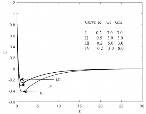
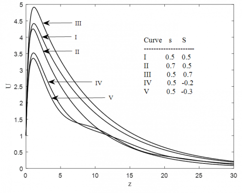
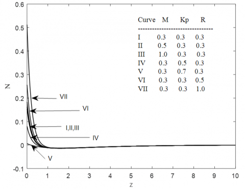
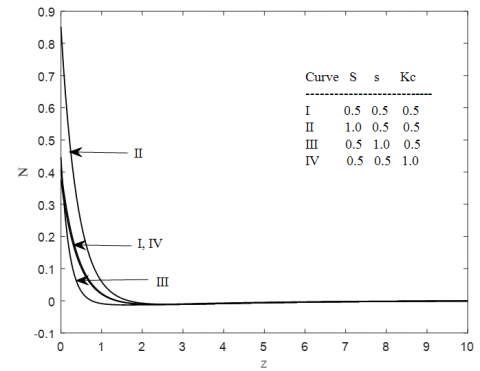
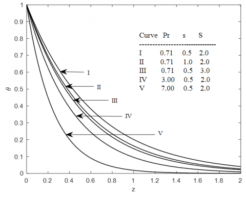
Figure 2 portrays the behavior of Prandtl number (Pr), magnetic (M) and permeability parameter (Kp) on the fluid momentum. Growth in the velocity of the polar fluid is marked with the increase in Prandtl number and porosity parameter. The expression of the Prandtl number reveals a relationship between the kinematic viscosities with thermal diffusivity, so attenuation in the thermal diffusivity is rendered that is dominated by the kinematic viscosity as Pr increases resulted in to increase in the fluid velocity. From the figure it is observed that with the increase in magnetic parameter, the velocity of the fluid decreases. The appearance of transverse magnetic field sets up by the action of the Lorentz force that resists the fluid velocity. Figure 3 reveals the influence of rotational parameter(R), thermal Grashof number (Gr) and mass Grashof number (Gm) on the velocity distributions. Fluid velocity attenuates with the increasing values of both the buoyancy parameters Gr and Gm. The rotational parameter has no significant role on the fluid velocity and this may be attributed due the occurrence of the porous matrix. Figure 4 portrays the effect of suction parameter (s) and heat source parameter (S) on velocity profile. It is observed that with the increase in suction parameter, the velocity of the polar fluid decelerates. But in case of heat source the impact opposes it. On careful observation, it is marked that in case of source, the fluid velocity increases throughout the domain. But in case of sink, the velocity of the flow field increases for 0 < z <7.5, decreases for 7.5 < z <12.5, increases for 12.5 < z < 20 and then there is no change. This fluctuation in case of sink may be due to the porosity of the medium. Figure 5 shows the effect of magnetic parameter (M), prorosity parameter (Kp) and rotation parameter (R) on angular velocity. It is observed that the angular velocity retards with the enhancement in the porosity parameter whereas it favors in to rise as rotation parameter increases. But the magnetic parameter has very negligible effect on angular velocity. Figure 6 displays the effect of heat source parameter (S), suction parameter(s) and chemical reaction parameter (Kc) on angular velocity. The angular velocity increases with the increase in heat source parameter but decreases with the increase in suction parameter where as chemical reaction has very negligible effect. Figure 7 displays the behavior of thermal and Grashof numbers (Gr and Gm), and viscosity ratio ($\delta$) on angular velocity. It is interesting to note that with the increase in viscosity ratio, the angular velocity decreases whereas thermal and mass Grashof number has very negligible effect. Figure 8 illustrates the consequence of Prandtl number (Pr), suction (s) and heat source parameter (S) on the fluid temperature. From the figure it is observed that the temperature of the fluid decreases with the increase in suction parameter and heat source parameter. The fluid temperature attenuates with the enhancement in the Prandtl number. Moreover, the resulting factor leads to decelerate the thickness of the thermal boundary layer. Figure 9 exhibits the behavior of heavier species (Sc), suction parameter(s) and chemical reaction parameter(Kc) on the solutal transfer profile. The figure shows that the fluid concentration slower down with increasing in chemical reaction and suction parameter. Interestingly, the increase in Schmidt number also decelerates the concentration level of the polar fluid at all points within the flow domain. Therefore, it is to conclude that, heavier species have a greater impact to retard the polar fluid concentration.
Table 1. Validation for skin friction and Nusselt number
|
R |
Kc |
$\delta$ |
s |
Kp |
Cf Bakr[5] |
Cf Present |
$-{\theta }'(0)$ Bakr[5] |
$-{\phi }'(0)$ Present |
|
0.2 |
0.2 |
0.2 |
1.0 |
100 |
6.648 |
6.64832 |
3.5371 |
3.5371 |
|
0.4 |
0.01 |
0.2 |
1.0 |
100 |
3.917 |
3.91713 |
3.5371 |
3.5371 |
Table 2. Variation of skin friction, couple stress, Nusselt number and Sherwood number with different flow parameters (Fixed parameters Gm=2, Gr=10, M=0.2, Pr=0.71, S=10, Sc=016)
|
R |
Kc |
$\delta$ |
s |
Kp |
Cf |
Cw |
$-{\theta }'(0)$ |
$-{\phi }'(0)$ |
|
0.2 |
0.2 |
0.2 |
1.0 |
0.5 |
6.3740 |
13.2681 |
3.5371 |
0.2760 |
|
0.4 |
0.01 |
0.2 |
1.0 |
0.5 |
6.5008 |
13.5328 |
3.5371 |
0.1694 |
|
0.6 |
0.01 |
0.2 |
1.0 |
0.5 |
6.4072 |
13.3380 |
3.5371 |
0.1694 |
|
0.8 |
0.01 |
0.2 |
1.0 |
0.5 |
6.2872 |
13.0901 |
3.5371 |
0.1694 |
|
0.2 |
0.5 |
0.2 |
1.0 |
0.5 |
6.2213 |
12.9510 |
3.5371 |
0.3739 |
|
0.2 |
1.0 |
0.2 |
1.0 |
0.5 |
6.0652 |
12.6270 |
3.5371 |
0.4879 |
|
0.2 |
0.01 |
0.4 |
1.0 |
0.5 |
7.2664 |
12.8802 |
3.5371 |
0.1694 |
|
0.2 |
0.01 |
0.6 |
1.0 |
0.5 |
8.1088 |
12.4875 |
3.5371 |
0.1694 |
|
0.2 |
0.01 |
0.8 |
1.0 |
0.5 |
9.0389 |
12.2891 |
3.5371 |
0.1694 |
|
0.2 |
0.01 |
0.2 |
1.5 |
0.5 |
7.1414 |
22.2780 |
3.7393 |
0.2465 |
|
0.2 |
0.01 |
0.2 |
2.0 |
0.5 |
7.7878 |
32.3774 |
3.9510 |
0.3249 |
|
0.2 |
0.01 |
0.2 |
2.5 |
0.5 |
8.5354 |
44.3433 |
4.1720 |
0.4040 |
|
0.2 |
0.01 |
0.2 |
1.0 |
1.5 |
8.6856 |
18.0814 |
3.5371 |
0.1694 |
|
0.2 |
0.01 |
0.2 |
1.0 |
2.0 |
9.7250 |
20.2441 |
3.5371 |
0.1694 |
|
0.2 |
0.01 |
0.2 |
1.0 |
2.5 |
10.5993 |
22.0632 |
3.5371 |
0.1694 |
Figure 2. Effect of Pr, M and Kp on velocity profile
Figure 3. Effect of R, Gr and Gm on velocity profile
Figure 4. Effect of s and S on velocity profile
Figure 5. Effect of M, Kp and R on angular velocity
Figure 6. Effect of S, s and Kc on angular velocity
Figure 7. Effect of Gr, Gm and $\delta$ on angular velocity
Figure 8. Effect of Pr, s and S on temperature profile
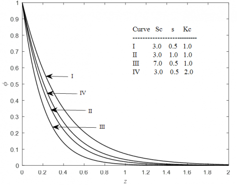
Figure 9. Effect of Sc, S and $\gamma$ on concentration profile
Table 2 shows the variation of shear stress at the plate i.e. skin friction (Cf), couple stress at the plate (Cw), rate of heat transfer at the plate i.e. Nusselt number (Nu) and the rate of mass transfer at the surface of the plate i.e. Sherwood number (Sh) with different flow parameters. From the table it is observed that, the rate coefficients i.e. skin friction and couple stress decreases with increasing rotation parameter whereas the rate of heat and solutal transfer remain unchanged. The increase in chemical reaction decelerates the skin friction and couple stress but impact is reversed for the Sherwood number whereas Nusselt number remains unchanged. The increase in microrotation favors in to boost up the skin friction but it retards the couple stress whereas the Nusselt number and Sherwood number remain unchanged. It is interesting to note that; suction parameter is favorable for the enhancement of all the engineering coefficients.
In the present study we have theoretically discussed the heat transfer phenomena on the time-dependent MHD flow of micropolar fluid in a porous medium within a rotating frame, considering oscillatory plate velocity with constant suction and first-order chemical reaction. The concluding remarks are:
|
x*,y*,z* |
dimensional co-ordinate axes |
|
z |
non-dimensional z-axis |
|
${{u}^{*}},{{v}^{*}},{{w}^{*}}$ |
velocity components towards x*,y*,z*- direction $[{{m}^{{}}}{{s}^{-1}}]$ |
|
t* |
dimensional time variable |
|
t |
non-dimensional time variable |
|
${{n}_{1}}^{*},{{n}_{2}}^{*}$ |
angular velocity components along x* and y* direction |
|
g |
acceleration due to gravity |
|
s |
suction parameter |
|
Cp |
specific heat $[Jk{{g}^{-1}}{{K}^{-1}}]$ |
|
B0 |
magnetic induction |
|
M |
non-dimensional magnetic parameter |
|
QH |
dimensional heat source |
|
S |
non-dimensional heat source |
|
D |
molecular diffusivity |
|
Kl |
dimensional chemical reactants |
|
Kc |
chemical reaction parameter |
|
T |
Fluid temperature $[{{m}^{2}}{{s}^{-1}}]$ |
|
R |
non-dimensional rotation parameter |
|
Ur |
uniform reference velocity |
|
Sc |
Schmidt number |
|
Pr |
Prandtl number |
|
K |
dimensional porosity parameter |
|
Kp |
non-dimensional porosity parameter |
|
Gr |
thermal Grashof number |
|
Gm |
mass Grashof number |
|
Greek symbols |
|
|
$\Omega $ |
dimensional rotation parameter |
|
$\beta$ |
volumetric thermal expansion |
|
$\hat{\beta}$ |
volumetric solutal expansion |
|
$\sigma$ |
electrical conductivity $\left[\Omega^{-1} m^{-1}\right]$ |
|
$\alpha$ |
rotational viscosity |
|
$\lambda^{*}$ |
dimensional micro-inertia density |
|
$\lambda$ |
non-dimensional micro-inertia density |
|
$\rho$ |
density of the fluid $\left[\mathrm{kgm}^{-3}\right]$ |
|
$\upsilon $ |
kinematic viscosity $\left[m^{2} s^{-1}\right]$ |
|
$\mu$ |
coefficient of viscosity $\left[\mathrm{kgm}^{-1} \mathrm{~s}^{-1}\right]$ |
|
$\delta$ |
viscosity ratio |
|
$\gamma$ |
material property |
${{B}_{1}}=(M+\frac{1}{Kp})+iR$ , ${{B}_{2}}=(M+\frac{1}{Kp})+i(R+n)$
${{B}_{3}}=(M+\frac{1}{Kp})+i(R-n)$ , ${{m}_{1}}=\frac{sSc+\sqrt{{{(sSc)}^{2}}+4KcSc}}{2}$ , ${{m}_{2}}=\frac{sPr+\sqrt{{{(sPr)}^{2}}+4S}}{2}$ , ${{m}_{3}}=\frac{s+\sqrt{{{s}^{2}}+4{{B}_{1}}(1+\delta )}}{2(1+\delta )}$ , ${{m}_{4}}=\frac{s+\sqrt{{{s}^{2}}+4in\lambda }}{2\lambda }$ , ${{m}_{5}}=\frac{s+\sqrt{{{s}^{2}}+4{{B}_{2}}(1+\delta )}}{2(1+\delta )}$ , ${{m}_{6}}=\frac{s+\sqrt{{{s}^{2}}-4in\lambda }}{2}$ , ${{m}_{7}}=\frac{s+\sqrt{{{s}^{2}}+4{{B}_{3}}(1+\delta )}}{2(1+\delta )}$ ,
${{A}_{1}}=\frac{-Gr}{(1+\delta ){{m}_{2}}^{2}-s{{m}_{2}}-{{B}_{1}}}$ , ${{A}_{2}}=\frac{-Gm}{(1+\delta ){{m}_{1}}^{2}-s{{m}_{1}}-{{B}_{1}}}$ , ${{h}_{1}}=\frac{i\delta s\lambda }{(1+\delta ){{s}^{2}}-\lambda {{s}^{2}}-{{B}_{1}}{{\lambda }^{2}}}$ ,
${{h}_{2}}=\frac{i({{A}_{1}}({{m}_{3}}-{{m}_{1}})+{{A}_{2}}({{m}_{3}}-{{m}_{2}})-{{m}_{3}})}{2-i{{h}_{1}}({{m}_{3}}-s/\lambda )}$ , ${{h}_{3}}={{h}_{2}}{{h}_{1}}$ , ${{A}_{3}}=1-{{A}_{1}}-{{A}_{2}}-{{h}_{3}}$ , ${{h}_{4}}=\frac{i\delta {{m}_{4}}}{(1+\delta ){{m}_{4}}^{2}-s{{m}_{4}}-{{B}_{2}}}$ , ${{h}_{5}}=\frac{i{{m}_{5}}}{2-i{{h}_{4}}({{m}_{5}}-{{m}_{4}})}$ , ${{h}_{6}}={{h}_{4}}{{h}_{5}}$ , ${{A}_{4}}=1-{{h}_{6}}$ , ${{h}_{7}}=\frac{i\delta {{m}_{6}}}{(1+\delta ){{m}_{6}}^{2}-s{{m}_{6}}-{{B}_{3}}}$ , ${{h}_{8}}=\frac{i{{m}_{7}}}{2-i{{h}_{7}}({{m}_{7}}-{{m}_{6}})}$, ${{h}_{9}}={{h}_{7}}{{h}_{8}}$ , ${{A}_{5}}=1-{{h}_{9}}$ .
[1] Eringen, A.C. (1966). Theory of micropolar fluids. Journal of Mathematics and Mechanics, 16(1): 1-18. http://dx.doi.org/10.1512/iumj.1967.16.16001
[2] Eringen, A.C. (1972). Theory of thermomicrofluids. Journal of Mathematical Analysis and Applications, 38: 480-496. https://doi.org/10.1016/0022-247X(72)90106-0
[3] Ariman, T., Turk, M.A., Sylvester, N.D. (1973). Microcontinuum fluid mechanics. International Journal of Engineering Science, 11(8): 905-9330. https://doi.org/10.1016/0020-7225(73)90038-4
[4] Ariman, T., Turk, M.A., Sylvester, N.D. (1974). Applications of microcontinuum fluid mechanics. International Journal of Engineering Science, 12(4): 273-293. https://doi.org/10.1016/0020-7225(74)90059-7
[5] Bakr, A.A. (2011). Effects of chemical reaction on MHD free convection and mass transfer flow of a micropolar fluid with oscillatory plate velocity and constant heat source in a rotating frame of reference. Commun Nonlinear Sci Numer Simulat, 16: 698-710. https://doi.org/10.1016/j.cnsns.2010.04.040
[6] Hussanan, A., Salleh, M.Z., Khan, I., Tahar, R.M. (2018). Heat and mass transfer in a micropolar fluid with Newtonian heating: An exact analysis. Neural Computing and Applications, 29(6): 59-67. https://doi.org/10.1007/s00521-016-2516-0
[7] Sheri, S.R, Shamshuddin, M.D. (2015). Heat and mass transfer on the MHD flow of micropolar fluid in the presence of viscous dissipation and chemical reaction. Procedia Engineering, 127: 885-892. https://doi.org/10.1016/j.proeng.2015.11.426
[8] Rout, P.K., Sahoo, S.N., Dash, G.C., Mishra, S.R. (2016). Chemical reaction effect on MHD free convection flow in a micropolar fluid. Alexandria Engineering Journal, 55: 2967-2973. https://doi.org/10.1016/j.aej.2016.04.033
[9] Animasaun, I.L. (2017). Melting heat and mass transfer in stagnation point micropolar fluid flow of temperature dependent fluid viscosity and thermal conductivity at constant vertex viscosity. Journal of the Egyptian Mathematical Society, 25(1): 79-85. https://doi.org/10.1016/j.joems.2016.06.007
[10] Mahmoud, M.A.A. (2010). Chemical reaction and variable viscosity effects on flow and mass transfer of a non-Newtonian viscoelastic fluid past a stretching surface embedded in a porous medium. Meccanica 45: 835-846. https://doi.org/10.1007/s11012-010-9292-1
[11] Khan, M. (2007). Partial slip effects on the oscillatory flows of a fractional Jeffrey fluid in a porous medium. Journal of Porous Media, 10(5): 473-488. https://doi.org/10.1615/JPorMedia.v10.i5.50
[12] Dessie, H., Kishan, N. (2014). MHD effects on heat transfer over stretching sheet embedded in porous medium with variable viscosity, viscous dissipation and heat source/sink. Ain Shams Engineering Journal, 5: 967-977. https://doi.org/10.1016/j.asej.2014.03.008
[13] Mishra, S.R., Pattnaik, P.K., Bhatti, M.M., Abbas, T. (2017). Analysis of heat and mass transfer with MHD and chemical reaction effects on viscoelastic fluid over a stretching sheet. Indian Journal of Physics, 91(10): 1219-1227. https://doi.org/10.1007/s12648-017-1022-2
[14] Mishra, S.R., Khan, I., Al-mdallal, Q.M., Asifa, T. (2018). Free convective micropolar fluid flow and heat transfer over a shrinking sheet with heat source. Case Studies in Thermal Engineering, 11: 113-119. https://doi.org/10.1016/j.csite.2018.01.005
[15] Mishra, S.R., Mohanty, J., Das, J.K. (2018). Free convective flow, heat and mass transfer of a micropolar fluid over a shrinking sheet in the presence of heat source. J. Eng. Phy. and Thermophys., 91(4): 983-990. https://doi.org/10.1007/s10891-018-1824-x
[16] Mishra, S.R., Tripathy, R.S., Dash, G.C. (2018). MHD viscoelastic fluid flow through porous medium over a stretching sheet in the presence of non-uniform heat source/sink. Rendiconti del Circolo Matematico di Palermo Series 2, 67(1): 129-143. https://doi.org/10.1007/s12215-017-0300-3
[17] Ganapathy, R.A. (1994). A note on oscillatory Couette flow in a rotating system. ASME J Appl Mech, 61(1): 208-209. https://doi.org/10.1115/1.2901403