Hojjat Ghorbani | Yaghoub Mahmoudi* | Farhad Dastmalchi Saei
© 2020 IIETA. This article is published by IIETA and is licensed under the CC BY 4.0 license (http://creativecommons.org/licenses/by/4.0/).
OPEN ACCESS
In this paper, we introduce a method based on Radial Basis Functions (RBFs) for the numerical approximation of Mathieu differential equation with two fractional derivatives in the Caputo sense. For this, we suggest a numerical integration method for approximating the improper integrals with a singularity point at the right end of the integration domain, which appear in the fractional computations. We study numerically the affects of characteristic parameters and damping factor on the behavior of solution for fractional Mathieu differential equation. Some examples are presented to illustrate applicability and accuracy of the proposed method. The fractional derivatives order and the parameters of the Mathieu equation are changed to study the convergency of the numerical solutions.
radial basis functions, fractional Caputo derivative, Mathieu differential equation
Differential equations explain mathematically most of physical phenomena such as electromagnetic, elastic wave equations, frequency modulation, parametric oscillators, mirror trap for neutral particles, motion of a quantum particles in a periodic potential [1], and a lot more. Mathieu differential equation
${{D}^{2}}y(t)+[a-2qcos(2t)]y(t)=0, y(0)=\underline{y}, y'(0)=\overline{y}$ (1)
is a famous differential equation which appears to describe such phenomena [2]. In Eq. (1) $a$ is the characteristic number and q is the characteristic parameter of the equation. The French mathematician Mile Lonard Mathieu introduced this equation for the first time and lately this equation was named in his honor the Mathieu equation [3]. The equation was formulated to describe the vibration modes of an elliptical membrane [2], but it has been applied to quadrupole ion traps theory in chemistry [4, 5], ultra cold atoms [6], models of quantum rotor [7], inverted pendulum, vibrations in an elliptic drum, stability of a floating body and Paul trap for charged particles [8, 9].
A simple harmonic oscillator obtains in Eq. (1) when we put q=0, It is well known that this oscillator performs free vibrations around the stable equilibrium position y=0. For $q\ne 0$ the Mathieu Eq. (1) may have a stable solution (when the motion is bounded) or unstable solution (when the motion is unbounded). The occurrence of one of these two outcomes depends on the combination of the parameters q and $a$. When presented graphically, this gives the so-called stability chart with regions of stability and regions of instability separated by the so-called transition curves, enabling one to clearly determine the resulting behavior and the stability property mentioned. This was extensively studied by Rand et al. [10] for classical damped Mathieu equation and fractional Mathieu equation with one fractional derivative.
The asymptotic solutions and transition curves for the generalized form of the non-homogeneous Mathieu differential equation are investigated in the paper [11]. An efficient numerical scheme is proposed for obtaining the stability charts for Mathieu equation by authors [12]. The existence of periodic and quasiperiodic solutions for generalized Van der Pol-Mathieu differential equation is proved using the averaging method in the paper [13]. Kovacic et al. provided a systematic overview of the methods to determine the corresponding stability chart of the classical Mathieu’s equation [14].
Mathieu equation is especially important to the theory of Josephson junctions, where it is equivalent to Schrödinger’s equation. Recently Wilkinson et al. [15] collected various approximations which appear throughout the physics and mathematics literature and examined their accuracy and regimes of applicability.
The fractional calculus is very popular and applicable tool to describe different phenomena these days. The memory and hereditary properties of various materials and processes were considered by the models based on fractional derivatives, where as in integer order models, such types of aspects are not considered. These leads fractional calculus to become an increasingly important topic in the literature of applied mathematics, engineering and other fields. For detailed definitions and theorems on fractional calculus and applications, the readers are referred to the Ref. [16].
Adding the term $^{C}{{D}^{\alpha }}y(t)$ in (1), which denotes the Caputo fractional derivative of function y of order $\alpha $, we obtain the fractional Mathieu differential equation as follows [10]:
${{D}^{2}}y(t)+\kappa {{ }^{C}}{{D}^{\alpha }}y(t)+[a-2qcos(2t)]y(t)=0, 0<\alpha \le 1,$ (2)
where, $\kappa $ is a constant. The general fractional form of Mathieu Eq. (2) is as follows:
$^{C}{{D}^{\beta }}y(t)+{{\kappa }^{C}}{{D}^{\alpha }}y(t)+[a-2qcos(2t)]y(t)=f(t),$ (3)
where,$0<\alpha \le 1$ and $1<\beta \le 2$, are fractional derivatives. Setting $\alpha =1$ and $\beta =2$ in (3), leads to the familiar damped Mathieu equation.
Fractional Mathieu equation is solved numerically by many scientists. For example, authors [10] have used the harmonic balance method. The Adomian decomposition and the series method were used in the paper [17] for fractional Mathieu equation with damped term. Najafi et al. have used the generalized differential transform method [18]. The dynamics of Mathieu equation with two kinds of van der Pol (VDP) fractional-order terms is investigated by Wen et al. [19]. Recently the Block-Pulse wavelets approximation method [20] was used by Pirmohabbati et al. for numerical solution of fractional Mathieu equation.
The Radial Basis Functions (RBF) method was introduced by Hardy [21] in 1971. At first, it was popular in multivariate interpolation [22]. In 1990, Kansa introduced a new method to use RBFs for solving parabolic, hyperbolic, and elliptic partial differential equations [23]. After that, radial basis functions have been widely applied in different fields of computational science.
In this paper, we use Radial Basis Functions (RBFs) to solve numerically the general fractional Mathieu differential Eq. (3). The results of this paper are compatible with those in the papers [10, 20] and other literatures. The rest of this paper is organized as follows. In Section 2, we review some basic definitions of fractional calculus and Radial Basis Functions. We also introduce a composite Simpson's numerical scheme for the improper integrals with a singularity at the right endpoint of the integration domain. In Section 3, we present the new numerical algorithm for solving fractional Mathieu equation. In Section 4, some examples are presented to illustrate the numerical method. Finally, we give conclusions in Section 5.
2.1 Fractional calculus
In this part a brief description of Riemann-Liouville and Caputo fractional integrals and derivatives are presented.
Definition 2.1: 1 The Riemann-Liouville fractional integration of order $\alpha (\alpha \in {{R}^{+}})$ is expressed by [16],
$\left\{ \begin{array}{*{35}{l}} _{0}I_{x}^{\alpha }f(x)=\frac{1}{\Gamma (\alpha )}\int_{0}^{x}{}{{(x-\tau )}^{\alpha -1}}f(\tau )d\tau ,\quad \quad & \alpha >0, \\ {} & {} \\ _{0}I_{x}^{0}f(x)=f(x), & \alpha =0, \\\end{array} \right.$ (4)
where, $\Gamma (\alpha )=\int_{0}^{\infty }{}{{x}^{\alpha -1}}{{\text{e}}^{-x}}\ dx$ is the well-known gamma function. This to end for simplicity we omit 0 and x in the fractional integration notation.
The operator ${{I}^{\alpha }}$ satisfies the following relations,
${{I}^{\alpha }}{{I}^{\gamma }}f(x)={{I}^{\alpha +\gamma }}f(x),$
${{I}^{\alpha }}{{I}^{\gamma }}f(x)={{I}^{\gamma }}{{I}^{\alpha }}f(x),$
$_{0}I_{x}^{\alpha }{{x}^{b}}=\frac{\Gamma (b+1)}{\Gamma (b+1+\alpha )}{{x}^{b+\alpha }}.$
Definition 2.2: 2 The Riemann-Liouville fractional derivative of order $\alpha $ of f(x) is defined as [16],
$_{0}^{RL}D_{x}^{\alpha }f(x)=\frac{1}{\Gamma (n-\alpha )}\frac{{{d}^{n}}}{d{{x}^{n}}}\int_{0}^{x}{}\frac{f(\tau )}{{{(x-\tau )}^{\alpha -n+1}}}d\tau ,$ (5)
where, $n-1<\alpha \le n$, $n\in N$.
Definition 2.3: 3 The Caputo fractional derivative so that $n-1<\alpha <n$ are expressed as [16],
$_{0}^{C}D_{x}^{\alpha }f(x)=\frac{1}{\Gamma (n-\alpha )}\int_{0}^{x}{}\frac{{{f}^{(n)}}(\tau )}{{{(x-\tau )}^{\alpha -n+1}}}d\tau .$ (6)
The main properties of the operator $_{0}^{C}D_{x}^{\alpha }$ are [16],
$_{0}^{C}D{{_{x}^{\alpha }}_{0}}I_{x}^{\alpha }f(x)=f(x),$ (7)
${ }_{0} I_{x}^{\alpha}{ }_{0}^{C} D_{x}^{\alpha} f(x)=f(x)-\sum_{j=0}^{n-1} f^{(j)}\left(0^{+}\right) \frac{x^{j}}{j !}$, (8)
$_{0}^{C}D_{x}^{\alpha }{{x}^{j}}=\left\{ \begin{array}{*{35}{l}} 0 & j\in {{N}_{0}}\ and\ j<n, \\ {} & {} \\ \frac{\Gamma (j+1)}{\Gamma (j+1-\alpha )}{{x}^{j-\alpha }} & j\notin {{N}_{0}}\ or\ j\ge n, \\\end{array} \right.$ (9)
where, ${{N}_{0}}=\{0,1,2,...\}$. The Caputo fractional derivative (6) is determined by Riemann-Liouville fractional derivative (5) as follows [16],
$_{0}^{C}D_{x}^{\alpha }f(x)=_{0}^{RL}D_{x}^{\alpha }f(x)-\sum\limits_{i=0}^{n-1}{}\frac{{{f}^{(i)}}(0)}{\Gamma (i+1-\alpha )}{{x}^{i-\alpha }},$ (10)
Accordingly, if ${{f}^{(i)}}(0)=0,\ i=0,1,...,n-1,$ then $_{0}^{C}D_{x}^{\alpha }f(x)$ and $_{0}^{RL}D_{x}^{\alpha }f(x)$ are equivalent.
2.2 Review of interpolation by RBFs
In this subsection, we briefly introduce the Radial Basis Functions. We state the relevant basic definitions and refer to the literatures (for example [24, 25]) for more details.
A function $K:{{R}^{d}}\times {{R}^{d}}\to R$ is symmetric, if$K(x,y)=K(y,x)$ holds for all $x, y\in {{R}^{d}}$. For scattered nodes ${{x}_{1}},\ldots ,{{x}_{n}}\in {{R}^{d}}$, the translates ${{K}_{j}}(x)=K({{x}_{j}},x)$ are called the trial functions.
Radial kernel is defined as:
$K(x, y)=\phi(r), r=\|x-y\|, x, y \in R^{d}$, (11)
where, $\phi$ :[0,\infty )\to R,$ is a scalar function. The function $\varphi $ is called a radial basis function. One can scale the kernels on Rd by a positive factor c which is called shape parameter. The accuracy of numerical solution and the condition number of collocation matrix are affected by the shape parameter c. There are some numerical methods for finding an appropriate parameter c to control the accuracy of the solution as well as conditioning of the collocation matrix. By importing the shape parameter c, the new scaled kernel is given by:
${{K}_{c}}(x,y)=K(\frac{x}{c},\frac{y}{c}), \forall x,y\in {{R}^{d}}.$ (12)
The scaled radial kernels on Rd is defined as
${{K}_{c}}(x,y)=\varphi (\frac{r}{c}), r=\left\| x-y \right\|, x,y\in {{R}^{d}}.$ (13)
Table 1 represents the most commonly used global RBFs $\varphi (r)$, where $n, \beta $ are RBF parameters and c is shape parameter.
Table 1. Global RBFs
|
Name |
$\varphi (r)$ |
Condition |
|
Gaussian(GS) |
${{e}^{-{{(cr)}^{2}}}}$ |
|
|
Multi quadric(MQ) |
${{(1+{{(cr)}^{2}})}^{\beta /2}}$ |
$\beta \ne 0, \beta \notin 2N$ |
|
Inverse quadric(IQ) |
${{(1+{{(cr)}^{2}})}^{-1}}$ |
|
|
Powers |
${{r}^{\beta }}$ |
$0\le \beta \notin 2N$ |
|
Thin-plate splines |
${{r}^{2n}}ln(r)$ |
$n\in N$ |
Yoon [24] showed that applying RBFs in Sobolov space has exponential convergence. Fornberg et al. [25] proved the spectral convergence of the method in the limit of flat RBFs. Madych has proved in the paper [26] that under certain conditions the interpolation error is $\varepsilon =O({{\lambda }^{c/h}})$ where h is the mesh size, and $0<\lambda <1$ is a constant. He presented that, there are two ways to improve the approximation, by reducing the size of h and by increasing the size of c. It means that if $c\to \infty $ then $\varepsilon \to 0$. While reducing h leads to the heavy computations, increasing c is without the extra computational cost, but it was proven in the paper [26] that as the error becomes smaller, the matrix becomes more ill-conditioned; hence the solution will break down as $c$ becomes too large. So, if the ill-conditioned system could be solved, h could be increased to obtain the best approximation.
Selecting the appropriate c affects the accuracy and convergence properties of RBFs. Optimal choice of c is still an open problem and lots of papers have been published in this area. We refer the readers to the papers [26-30] for more details.
In this study, we select$c$through our numerical observation such that the stability of the proposed method is achieved.
2.3 Composite rule for singular integrals
In this subsection a composite Simpson's numerical scheme is provided for integrals with a singularity at the right endpoint of the integration domain [31].
The improper integral with a singularity at the right endpoint,
$\int_{a}^{b}{}\frac{dt}{{{(b-t)}^{q}}},$ (14)
converges if and only if $0<q<1$, and in this case, one defines,
$\int_{a}^{b}{}\frac{dt}{{{(b-t)}^{q}}}=\frac{{{(b-a)}^{1-q}}}{1-q}.$ (15)
Let g is continuous on $[a,b]$, then the improper integral
$\int_{a}^{b}{}\frac{g(t)}{{{(b-t)}^{q}}}dt,$ (16)
exists, where $0<q<1$. This integral can be approximated with Composite Simpson’s rule. For this we assume that $g\in {{C}^{5}}[a,b]$. In this case, the fourth order Taylor polynomial, ${{P}_{4}}(t)$, for g about b is constructed as:
${{P}_{4}}(t)=g(b)-{g}'(b)(b-t)+\frac{{{g}'}'(b)}{2!}{{(b-t)}^{2}}-\frac{{{g}^{(3)}}(b)}{3!}{{(b-t)}^{3}}+\frac{{{g}^{(4)}}(b)}{4!}{{(b-t)}^{4}}.$ (17)
Then we can write,
$\int_{a}^{b}{}\frac{g(t)}{{{(b-t)}^{q}}}dt=\int_{a}^{b}{}\frac{g(t)-{{P}_{4}}(t)}{{{(b-t)}^{q}}}dt+\int_{a}^{b}{}\frac{{{P}_{4}}(t)}{{{(b-t)}^{q}}}dt.$ (18)
P4(x) is a polynomial, then the first integral in (18) can be exactly determined by:
$\begin{array}{*{35}{l}} \int_{a}^{b}{}\frac{{{P}_{4}}(t)}{{{(b-t)}^{q}}}dt & =\sum\limits_{k=0}^{4}{}{{(-1)}^{k}}\int_{a}^{b}{}\frac{{{g}^{(k)}}(b)}{k!}{{(b-t)}^{k-q}}dt \\ {} & =\sum\limits_{k=0}^{4}{}{{(-1)}^{k}}\frac{{{g}^{(k)}}(b)}{k!(k+1-q)}{{(b-a)}^{k+1-q}}. \\\end{array}$ (19)
When the Taylor polynomial P4(t) is too close to g(x) throughout the interval $[a,b]$, (19) is the dominant part of the approximation. We must add to this value the following approximation,
$\int_{a}^{b}{}\frac{g(t)-{{P}_{4}}(t)}{{{(b-t)}^{q}}}dt.$
To this, we first define the function G(t) as follows
$G(t)=\left\{ \begin{matrix} \frac{g(t)-{{P}_{4}}(t)}{{{(b-t)}^{q}}} & a\le t<b \\ 0 & t=b \\\end{matrix} \right.$
G(t) is a continuous function on $[a,b]$. Because, $0<q<1$ and $P_{4}^{(k)}(b)={{g}^{(k)}}(b)$ for $k=0,1,2,3,4$, so $G\in {{C}^{4}}[a,b]$. Therefore, we can use the Composite Simpson’s rule to approximate the integral of G on $[a,b]$. Adding this to the value in Eq. (19) gives an approximation to the improper integral (18), with the accuracy of the Composite Simpson’s rule approximation (which is of order $O({{h}^{4}})$for any given step length (h). The function $SINGSIMP(g,a,b,q,\varepsilon )$approximates (16) with the accuracy of $\varepsilon $ (see Appendix 1).
To solve the general Mathieu Eq. (3) with the initial conditions $y(0)=\underline{y}, {y}'(0)=\overline{y}$ on the interval $[0,T]$, we set:
$y(t)=\sum\limits_{j=1}^{N}{}{{y}_{j}} {{\varphi }_{j}}(t)={{\Phi }^{T}}(t)Y,$ (20)
where,
$\begin{align} & \Phi (t)={{\left[ {{\varphi }_{1}}(t),{{\varphi }_{2}}(t),\ldots ,{{\varphi }_{N}}(t) \right]}^{T}}, \\ & Y=[{{y}_{1}},{{y}_{2}},\ldots ,{{y}_{N}}{{]}^{T}}, \\ \end{align}$ (21)
are RBF basis vector and coefficients vector respectively and ${{\varphi }_{j}}(t)=\varphi (|t-{{t}_{j}}|), j=1,2,\ldots ,N$ are RBF basis functions and ${{t}_{1}},{{t}_{2}},\ldots ,{{t}_{N}}$ are arbitrary (not necessary equally spaced) points of $[0,T]$. Differentiating (20) of order $\alpha $and β in the fractional Caputo scene, we get
$_{0}^{C}D_{t}^{\alpha }y(t)=\sum\limits_{j=1}^{N}{}{{y}_{j}} _{0}^{C}D_{t}^{\alpha }{{\varphi }_{j}}(t)=\Phi _{\alpha }^{T}(t)Y,$ (22)
$_{0}^{C}D_{t}^{\beta }y(t)=\sum\limits_{j=1}^{N}{}{{y}_{j}} _{0}^{C}D_{t}^{\beta }{{\varphi }_{j}}(t)=\Phi _{\beta }^{T}(t)Y,$ (23)
where,
${{\Phi }_{\alpha }}(t)={{\left[ _{0}^{C}D_{t}^{\alpha }{{\varphi }_{1}}(t),_{0}^{C}D_{t}^{\alpha }{{\varphi }_{2}}(t),\ldots ,_{0}^{C}D_{t}^{\alpha }{{\varphi }_{N}}(t) \right]}^{T}},$
and
${{\Phi }_{\beta }}(t)={{\left[ _{0}^{C}D_{t}^{\beta }{{\varphi }_{1}}(t),_{0}^{C}D_{t}^{\beta }{{\varphi }_{2}}(t),\ldots ,_{0}^{C}D_{t}^{\beta }{{\varphi }_{N}}(t) \right]}^{T}}.$
Substituting (20), (22) and (23) in (3) we get:
$\left( \Phi _{\beta }^{T}(t)+\kappa \ \Phi _{\alpha }^{T}(t)+(a-2qcos2t)\,{{\Phi }^{T}}(t) \right)\,Y=f(t).$ (24)
Now we choose $N-2$ distinct collocation points ${{x}_{1}},{{x}_{2}},\ldots ,{{x}_{N-2}}\in [0,T]$ and collocate (24) as follows:
$\left( \Phi _{\beta }^{T}({{x}_{i}})+\kappa \,\Phi _{\alpha }^{T}({{x}_{i}})+(a-2qcos2{{x}_{i}}){{\Phi }^{T}}({{x}_{i}}) \right)Y=f({{x}_{i}}), i=1,2,\ldots ,N-2.$ (25)
Finally, we summarize (25) as the following matrix form:
$\left( A+\kappa \,B+C \right)\,Y=F,$ (26)
where,
$\begin{matrix} {{A}_{ij}}=_{0}^{C}D_{t}^{\beta }{{\varphi }_{j}}(t{{)|}_{t={{x}_{i}}}}, \\ {{B}_{ij}}=_{0}^{C}D_{t}^{\alpha }{{\varphi }_{j}}(t{{)|}_{t={{x}_{i}}}}, \\ {{C}_{ij}}=(a-2qcos2{{x}_{i}}){{\varphi }_{j}}({{x}_{i}}), \\ {{F}_{i}}=f({{x}_{i}}), \\\end{matrix}$ (27)
for $i=1,2,\ldots ,N-2$,$j=1,2,\ldots ,N$. (26) is a system of $(N-2)\times N$ linear equations. Together with two initial conditions,
$y(0)=\underline{y}$ (28)
${y}'(0)=\overline{y}$ (29)
we get a system of N linear equations of N unknown coefficients ${{y}_{1}},{{y}_{2}},\ldots ,{{y}_{N}}$. In (29) ${{\Phi }_{1}}(t)$ denotes the first derivative of vector function $\Phi (t).$
Now we write the final linear equation as follows:
$M\,Y=Z,$ (30)
where,
$\begin{align} & {{M}_{ij}}={{A}_{ij}}+\kappa \,{{B}_{ij}}+{{C}_{ij}},\quad i=1,2,...,N-2\text{ , } \\ & {{M}_{N-1\,j}}={{\varphi }_{j}}(0),\quad \quad \quad \ j=1,2,...N,\quad \\ & {{M}_{Nj}}=\varphi {{'}_{j}}(0), \\ \end{align}$ (31)
and
$\begin{align} & {{Z}_{i}}={{F}_{i}},\quad \quad i=1,2,...,N-2\text{ , } \\ & {{Z}_{N-1}}=\underline{y},\quad \\ & {{Z}_{N}}=\overline{y}. \\ \end{align}$ (32)
Here we must emphasize that the matrix components ${{A}_{ij}}$ and ${{B}_{ij}}$ are as follows
$\begin{align} & {{A}_{ij}}=_{0}^{C}D_{t}^{\beta }{{\varphi }_{j}}(t{{)|}_{t={{x}_{i}}}} \\ & \quad \ =\frac{1}{\Gamma (2-\beta )}\int_{0}^{{{x}_{i}}}{}{{({{x}_{i}}-\tau )}^{1-\beta }}{{{{{\varphi }'}'}}_{j}}(\tau )d\tau . \\ \end{align}$ (33)
$\begin{align} & {{B}_{ij}}=_{0}^{C}D_{t}^{\alpha }{{\varphi }_{j}}(t{{)|}_{t={{x}_{i}}}} \\ & \quad \,\,\,=\frac{1}{\Gamma (1-\alpha )}\int_{0}^{{{x}_{i}}}{}{{({{x}_{i}}-\tau )}^{-\alpha }}{{{{\varphi }'}}_{j}}(\tau )d\tau . \\ \end{align}$ (34)
Since $0<\alpha <1$ and $1<\beta <2$ then both improper integrals (33) and (34) are convergent and can be approximated by composite Simpson's method as mentioned in section 2.
The algorithm of this method is given as follows:
Algorithm 1.
1. choose $\ \phi (t),\ T,N,\varepsilon $
2. set $h=T/(N-1)$
3. set ${{t}_{j}}=(j-1)h,\ \ j=1,2,...,N$
4. set ${{\phi }_{j}}(t)=\phi (|t-{{t}_{j}}|),\ j=1,2,...,N$
5. set ${{x}_{k}}=(k-1/2)h,\ k=1,2,...,N-1$
6. for $i=1:N-2$
for $j=1:N$
$A_{ij}^{{}}=SINGSIMP(\phi '{{'}_{j}}(t),0,{{x}_{i}},\beta -1,\varepsilon )/\Gamma (2-\beta )$
$B_{ij}^{{}}=SINGSIMP(\phi {{'}_{j}}(t),0,{{x}_{i}},\alpha ,\varepsilon )/\Gamma (1-\alpha )$
${{C}_{ij}}=(a-2qcos2{{x}_{i}}){{\varphi }_{j}}({{x}_{i}})$
${{M}_{ij}}={{A}_{ij}}+\kappa \,{{B}_{ij}}+{{C}_{ij}}$
end
${{Z}_{i}}=f({{x}_{i}})$
end
7. for $j=1:N$
${{M}_{N-1\,j}}={{\varphi }_{j}}(0)$
${{M}_{Nj}}=\varphi {{'}_{j}}(0)$
end
8. ${{Z}_{N-1}}=\underline{y}\quad $
9. solve MY=Z
10. set $y(t)=\sum\limits_{j=1}^{N}{}{{y}_{j}} {{\varphi }_{j}}(t)$
In this section, in order to test the numerical method, we present some illustrative examples. We use different values of $\alpha , \beta , \kappa , q, a$ and f and plot the achieved numerical solutions and compare them with each other and the results obtained by Pirmohabbati et al. [20]. When $0<\alpha <1$ and $1<\beta <2$, the Mathieu equation is of fractional order. In this case there is no known analytic solution for Mathieu equation so the results are compared with the case that the orders are integer. By numerical experiments we choose the shape parameter c=h, where c is RBF parameter and hare the mesh size. The computations are performed by Maple 16 with 40 digits of computation. The Condition number of coefficient matrix are often in the domain ${{[10}^{10}}{{,10}^{20}}]$. We study (3) in three different cases.
Case A: In (3), we set $\kappa =1$, $a=1$ and q=0, with initial values $y(0)=1$ and ${y}'(0)=-1$and$f(t)={{e}^{-t}}$where the exact solution is $y(t)={{e}^{-t}}$.
Table 2 presents the numerical results for different RBFs with $T=1,\ \beta =2$, $\alpha =1$ and $c=h$. As we see in Table 2, the error norms highly affected by increasing N.
In Table 3 we fixed h=0.1 and changed c=kh. The results for different RBFs show that L2 norm decreases as c increases.
The numerical solution with $\beta =2$, $\alpha =1$ and the exact solution $y(t)={{e}^{-t}}$ are plotted in Figure 1. The graph of absolute error with $\beta =2$, $\alpha =1$ is represented in Figure 2.
Table 2. The ${{L}_{\infty }}$ and L2 norm for different values of N
|
RBFs |
N |
${{L}_{\infty }}$ |
L2 |
|
GS |
5 |
1.2367e-2 |
2.6761e-3 |
|
10 |
3.1366e-8 |
3.1028e-9 |
|
|
20 |
1.7318e-14 |
2.4091e-16 |
|
|
40 |
5.4396e-21 |
2.7160e-23 |
|
|
MQ |
5 |
4.7986e-3 |
1.0433e-3 |
|
10 |
8.0846e-9 |
7.9907e-10 |
|
|
20 |
1.1441e-20 |
4.7918e-22 |
|
|
40 |
4.7918e-25 |
4.3043e-27 |
|
|
IQ |
5 |
1.0182e-2 |
2.1988e-3 |
|
10 |
1.5795e-8 |
1.5603e-9 |
|
|
20 |
1.6640e-21 |
7.2423e-23 |
|
|
40 |
4.2156e-26 |
2.2128e-28 |
Table 3. The affects of c=kh on L2for h=0.1
|
$k$ |
GS |
MQ |
IQ |
|
8 |
2.8127e-6 |
9.1934e-5 |
8.5498e-4 |
|
4 |
2.1802e-7 |
1.1431e-6 |
6.1748e-6 |
|
2 |
2.1937e-8 |
1.8897e-8 |
5.9586e-8 |
|
1 |
3.1028e-9 |
7.9907e-10 |
1.5603e-9 |
|
1/2 |
6.5205e-10 |
1.1637e-10 |
1.5880e-10 |
|
1/4 |
2.0685e-10 |
4.9421e-11 |
5.5103e-11 |
|
1/8 |
9.5615e-11 |
3.7367e-11 |
3.8537e-11 |
|
1/16 |
5.9532e-11 |
3.4397e-11 |
3.4898e-11. |
Figure 1. The graph of exact and approximate solution ($\beta =2, \alpha =1$) with $N=20$ for Case A
Figure 2. The graph of absolute error ($\beta =2, \alpha =1$) with $N=20$ for Case A
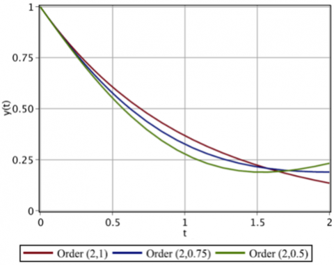
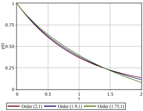
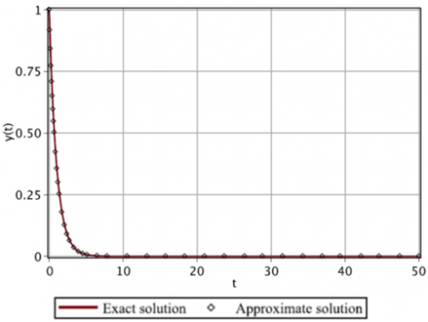
Now we keep $\beta =2$ fixed and change $\alpha =1$ to $\alpha =0.75$ and $\alpha =0.5$. Then we keep $\alpha =1$ and change $\beta =2$ to $\beta =1.9$ and $\beta =1.75$ respectively, which the results are plotted in Figures 3 and 4. The results show that the numerical solution converges in all the cases when $\beta $ and $\alpha $ are integer or rational numbers. To show the convergency of the approximate solution we plotted the exact and numerical solution with $\beta =2$ and $\alpha =1$ on the interval [0,50] in Figure 5.
Figure 3. The graph of approximate solution for $\beta =2$ and $\alpha =1, 0.75, 0.5$ with $N=20$ for Case A.
Figure 4. The graph of approximate solution for $\beta =2, 1.9, 1.75$ and $\alpha =1$ with $N=20$ for Case A.
Figure 5. The graph of exact solution $y(t)={{e}^{-t}}$ and approximate solution with $N=200$ for Case A.
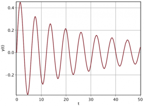
Case B: In (3), suppose $f(t)=0$, $\kappa =0$, $a=1$ and $q=0.1$, with initial values $y(0)=0$ and ${y}'(0)=0.5$. The numerical solution with $\alpha =1$, $\beta =2$ is plotted as follows as Figure 6. In fact, in this case we solve the Mathieu equation without damping term ($\kappa =0$). It is clear from Figure 6 that the solution diverges in this case. Our numerical solution is compatible with the results of the paper [20].
Figure 6. The graph of approximate solution for $\beta =2$, $\alpha =1$ and $N=200$ for Case B.
Figure 7. The graph of approximate solution for $\beta =2, 1.97, 1.95$ and $\alpha =1$ for Case B.
Figure 8. The graph of approximate solution for $\beta =1.9, 1.8, 1.7$ and $\alpha =1$ for Case B.
For the next attempt we keep $\alpha =1$ and the other coefficients fixed and then change $\beta $ from 2 to 1.97 and 1.95 (see Figure 7). The numerical results show that the solution is divergent. It is obvious from Figure 7 that when the derivatives occur with fractional order, the solution diverges faster and the divergency rate decreases as $\beta $ decreases.
Now we continue with $\alpha =1$ and other coefficients fixed and change $\beta $ from 2 to 1.9, 1.8 and 1.7. The results which were plotted in Figure 8 show that for these values of $\beta $ the behavior of numerical solution changes to convergency. Then we conclude that in the absence of damping term the solution of the Mathieu equations diverges for large values of $\beta $ ($\beta $ near to 2) and converges for smaller values of $\beta $.
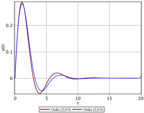
Case C: In (3), suppose $f(t)=0$, $\kappa =0.15$$a=1$ and $q=0.1$, with initial values $y(0)=0$ and ${y}'(0)=0.5$. The numerical solution with $\alpha =1$, $\beta =2$ is plotted in Figure 9. The numerical results of our method, which are compatible with those on the paper [20], show the convergency of the solution in this case.
Figure 9. The graph of approximate solution ($\beta =2,\ \alpha =1$) for Case C.
Figure 10. The graph of approximate solution for $\beta =2$ and $\alpha =0.9, 0.8$ for Case C.
Figure 11. The graph of approximate solution for $\beta =2, 1.97, 1.95$ and $\alpha =1$ for Case C.
Figure 12. The graph of approximate solution with fractional order of derivatives for Case C.
We keep $\beta =2$ and fix the other coefficients and change $\alpha $ from $1$ to $0.9$and $0.8$. The results plotted in Figure 10 show that the solution converges faster than the case that $\alpha =1$. If we keep $\alpha =1$ fixed and change $\beta $ from $2$ to $1.97$ and then $1.95$, the plots of results in Figure 11 show the convergency of the results which decays with decreasing of $\alpha $.
For the last attempt we change $\beta =2$ and $\alpha =1$ to $\beta =1.95$ and $\alpha =0.8$ first and then to $\beta =1.9$ and $\alpha =0.7$ which the graph is plotted in Figure 12.
In this work, the fractional Mathieu differential Eq. (3), including fractional order damping factor, was solved by using radial basis functions. Three classes of radial basis functions, the Gaussian (GS), multi quadric (MQ) and inverse quadric (IQ), have been used. Numerical results in all three classes converge to the solution of the equation. But the MQ and IQ classes are a little more accurate than GS. As N the number of radial basis functions increases, the approximation error decreases rapidly in all three cases, but the condition number of the required linear system increases rapidly. This requires that double accuracy of computation to be used.
By changing the characteristic parameters of the equation, the resulting numerical solutions in both stability and instability states converge to the exact solution of the Mathieu equation, which are compatible with the analytical and numerical results of other studies.
The function SINGSIMP(g, a, b, q, ε) approximates the singular integral,
$I=\int_{a}^{b}{}\frac{g(t)}{{{(b-t)}^{q}}}dt,$
with absolute error less than or equal to $\varepsilon $, where $0<q<1$ and g is a smooth function.
$function\quad SINGSIMP(g,a,b,q,\varepsilon )$
${{P}_{4}}(t)=\sum\limits_{k=0}^{4}{\frac{{{g}^{(k)}}(b)}{k!}{{(b-t)}^{k}}},$
${{I}_{1}}=\sum\limits_{k=0}^{4}{}{{(-1)}^{k}}\frac{{{g}^{(k)}}(b)}{k!(k+1-q)}{{(b-a)}^{k+1-q}}$
$G(t)=\left\{ \begin{matrix}\frac{g(t)-{{P}_{4}}(t)}{{{(b-t)}^{q}}} & a\le t<b \\ 0 & t=b \\\end{matrix} \right.$
${{M}_{4}}=\underset{a\le t\le b}{\mathop{\max }}\,\left| {{G}^{(4)}}(t) \right|,$
${{h}_{1}}={{\left( \frac{180\varepsilon }{(b-a){{M}_{4}}} \right)}^{1/4}},$
$N=2\left[ \frac{b-a}{2{{h}_{1}}} \right]+2,$
${{h}_{2}}:=\frac{b-a}{N},$
${{x}_{k}}=a+k{{h}_{2}},\quad \quad k=0,1,2,...,N$${{I}_{2}}=\frac{{{h}_{2}}}{3}\left( G({{x}_{0}})+4\sum\limits_{k=0}^{N/2-1}{G({{x}_{2k+1}})}+2\sum\limits_{k=1}^{N/2-2}{G({{x}_{2k}})}+G({{x}_{N}}) \right),$
$return\quad I={{I}_{1}}+{{I}_{2}},$
$end.$
[1] Slater, J. (1952). A soluble problem in energy bands. Phys. Rev., 87(5): 807.
[2] Mathieu, E. (1868). Memoire sur le movement vibratoire dune membrance de forme elliptique. Journal de Mathematiques Pures Appliqués, 13: 137-203.
[3] Duhem, P. (1892). Emile Mathieu, his life and works. Bull. Amer. Math., Soc., 1(7): 156-168. https://projecteuclid.org/euclid.bams/1183407338
[4] March, R. (1997). An introduction to quadrupole ion trap mass spectrometry. Journal of Mass Spectrometry, 1(7): 351-369. arXiv:1211.0050.
[5] Baranov, V. (2003). Analytical approach for description of ion motion in quadrupole mass spectrometer. Journal of the American Society for Mass Spectrometry, 14(8): 818-824. https://doi.org/10.1016/S1044-0305(03)00325-8
[6] Rey, A., Pupillo, G., Clark, C., Williams, C. (2005). Ultracold atoms confined in an optical lattice plus parabolic potential: A closed form approach. Phys. Rev., 72(3): 033616. https://doi.org/10.1103/PhysRevA.72.033616
[7] Ayub, M., Naseer, K., Ali, M., Saif, F. (2009). Atom optics quantum pendulum. J. Russ. Laser Res., 30(3): 205-223. https://doi.org/10.1007/s10946-009-9078-x
[8] Nwamba, J. (2013). Delayed Mathieu equation with fractional order damping an approximate analytical solution. International Journal of Mechanics and Applications, 3(4): 70-75. https://doi.org/10.5923/j.mechanics.20130304.02
[9] Stoker, J. (1950). Nonlinear Vibrations in Mechanical and Electrical Systems. Interscience Publishers, New York.
[10] Rand, R., Sah, S., Suchorsky, M. (2010). Fractional mathieu equation. Communications in Nonlinear Science and Numerical Simulation, 15(11): 3254-3262. https://doi.org/10.1016/j.cnsns.2009.12.009
[11] Younesian, D., Esmailzadeh, E., Sedaghati, R. (2007). Asymptotic solutions and stability analysis for generalized non-homogeneous Mathieu equation. Communications in Nonlinear Science and Numerical Simulation, 12(1): 58-71. https://doi.org/10.1016/j.cnsns.2006.01.005
[12] Bobryk, R.V., Chrzeszczyk, A. (2009). Stability regions for Mathieu equation with imperfect periodicity. Physics Letters A, 373(39): 3532-3535. https://doi.org/10.1016/j.physleta.2009.07.069
[13] Kalas, J., Kaderabek, K. (2014). Periodic solutions of a generalized Van der Pol-Mathieu differential equation. Applied Mathematics and Computation, 234: 192-202. https://doi.org/10.1016/j.amc.2014.01.161
[14] Kovacic, I., Rand, R., Sah, S.M. (2018). Mathieu’s equation and its generalizations: Overview of stability charts and their features. Applied Mechanics Reviews, 70(2): 020802. https://doi.org/10.1115/1.4039144
[15] Wilkinson, S.A., Vogt, N., Golubev, D.S., Cole, J.H. (2018). Approximate solutions to Mathieu’s equation. Physica E: Low-dimensional Systems and Nanostructures, 100: 24-30. https://doi.org/10.1016/j.physe.2018.02.019
[16] Podlubny, I. (1990). Fractional Differential Equations. San Diego, Academic Press.
[17] Abdelhalim, E., Elsayed, D.M., Aljoufi, M.D. (2012). Fractional calculus model for damped Mathieu equation: Approximate analytical solution. Applied Mathematical Science, 6(82): 4075-4080.
[18] Najafi, H., Mirshafaei, S., Toroqi, E. (2012). An approximate solution of the Mathieu fractional equation by using the generalized differential transform method (GDTM). Applications and Applied Mathematics, 7(1): 347-384.
[19] Wen, S., Shen, Y., Li, X., Yang, S. (2016). Dynamical analysis of Mathieu equation with two kinds of van der Pol fractional-order terms. International Journal of Non-Linear Mechanics, 84: 130-138. https://doi.org/10.1016/j.ijnonlinmec.2016.05.001
[20] Pirmohabbati, P., Sheikhani, A.R., Najafi, H.S., Ziabari, A.A. (2019). Numerical solution of fractional mathieu equations by using block-pulse wavelets. Journal of Ocean Engineering and Science, 4(4): 299-307. https://doi.org/10.1016/j.joes.2019.05.005
[21] Hardy, R. (1971). Multiquadratic equation of topology and other irregular surface. Journal of Geophysical Research, 76(8): 1905-1915. https://doi.org/10.1029/JB076i008p01905
[22] Buhmann, M. (1990). Multivariate interpolation in odd-dimensional Euclidean spaces using multiquadrics. Constructive Approximation, 6(1): 21-34. https://doi.org/10.1007/BF01891407
[23] Kansa, E. (1990). Multiquadricsa scattered data approximation scheme with applications to computational fluid-dynamics-II solutions to parabolic, hyperbolic and elliptic partial differential equations. Computers & Mathematics with Applications, 19(8-9): 147-161. https://doi.org/10.1016/0898-1221(90)90271-K
[24] Yoon, J. (1999). Spectral approximation orders of radial basis function interpolation on the Sobolov space. SIAM J. Math. Anal., 33(4): 946-958. https://doi.org/10.1137/S0036141000373811
[25] Fornberg, B., Wright, G., Larsson, E. (2004). Some observations regarding interpolants in the limit of flat radial basis functions. Comput. Math. Appl., 47(1): 37-55. https://doi.org/10.1016/S0898-1221(04)90004-1
[26] Madych, W. (1992). Miscellaneous error bounds for multiquadric and related interpolators. Computers & Mathematics with Applications, 24(12): 121-138. https://doi.org/10.1016/0898-1221(92)90175-H
[27] Haq, S., Hussain, M. (2018). Selection of shape parameter in radial basis functions for solution of time-fractional Black-Sholes models. Appl. Math. Comput., 335: 248-263. https://doi.org/10.1016/j.amc.2018.04.045
[28] Mongillo, M. (2011). Choosing basis functions and shape parameters for radial basis function methods. SIAM Undergrad. Res. Online, 190-209.
[29] Fallah, A., Jabbari, E., Babaee, R. (2019). Development of the Kansa method for solving seepage problems using a new algorithm for the shape parameter optimization. Comput. Math. Appl., 77(3): 815-829. https://doi.org/10.1016/j.camwa.2018.10.021
[30] Golbabai, A., Mohebianfar, E., Rabiei, H. (2015). On the new variable shape parameter strategies for radial basis functions. Computational and Applied Mathematics, 34(2): 691-704. https://doi.org/10.1007/s40314-014-0132-0
[31] Burden, R.L., Faires, J.D. (2010). Numerical Analysis. Richard Stratton Ninth Edition.