Samad Noeiaghdam* | Denis Sidorov
© 2020 IIETA. This article is published by IIETA and is licensed under the CC BY 4.0 license (http://creativecommons.org/licenses/by/4.0/).
OPEN ACCESS
The aim of this study, is to present the fractional model of energy supply-demand system (ES-DS) based on the Caputo-Fabrizio derivative. For the first time, the existence and uniqueness of solution of the fractional model of ES-DS are proved and it is the main novelty of this paper. Also, we know that the obtained results from mathematical models with fractional order are more accurate than usual models. This model is based on four important functions, energy resources demand (ERD) ε1, energy resource supply (ERS) ε2, energy resource import (ESI) ε3 and renewable energy resources (RER) ε4. Also, applying the obtained numerical results, we can forecast the rate of these functions for spacial interval of time.
fractional differential equations, energy supply-demand system, caputo-fabrizio derivative
Mathematical models play an important role in the analysis, behavior measurement and future prediction of various phenomena. Recently, many mathematical models have been presented in various fields. Yuzbasi et al. [1, 2] applied the exponential Galerkin method and Bessel collocation method for solving model of HIV infection of CD4+T cells. Also, Noeiaghdam and Khoshrouye Ghiasi [3, 4] discussed the homotopy analysis transform method to approximate both CD4+T and CD8+T-cells and Ahmad Naik et al. [5-7] studied the fractional model of HIV infection. Mathematical models of computer viruses were illustrated by Ozturk et al. [8] using Chebyshev polynomials and its fractional form was studied by Singh et al. [9] applying fractional derivative. Moreover the non-linear SIR model of computer viruses was solved by homotopy analysis method, variational iteration method and Adomian decomposition method [10-12]. Guerrero et al. [13] applied the homotopy analysis method and Sikander et al. [14] used the variation of parameter method for solving model of smoking habit and the model of tuberculosis infection is illustrated by Atangana-Baleanu derivative [15] and variable-order fractional derivatives [16]. For more mathematical models you can see ref. [17-20].
Energy is one of applicable fields that plays an important role in the economy of countries and human life. Many criteria and factors can affect the production and supply of energy. Therefore, the security of energy demand is one of the important issues that has been considered in recent years because it has a fundamental role in energy development. Since many factors can affect the ES-DS, this model is a complex and unstable system. But given the importance of energy supply and demand, controlling this system has always been of strategic importance. Therefore, in order to develop long-term, medium-term and short-term plans, accurate models are needed so that we can take control of the ES-DS with the necessary forecasts. Sun et al. [21] considered the time-delayed feedback control of the energy resource chaotic system. The energy resources demand-supply system and its dynamical analysis was illustrated by Sun and Tian [22]. Also, four-dimensional energy resources system was discussed with adaptive control and synchronization [23], with the model reference control [24] and with linear feedback control [25]. Moreover, supply-demand balancing renewable electricity using storage systems is one of the main challenges of contemporary power engineering. Sidorov et al. [26] considered application of integral equations for electric load leveling problems using storage systems.
Fractional calculus has real applications in different fields of engineering and sciences. Wang et al. [27] applied the fractional calculus for image denoising, Chen et al. [28] combined the application of blockchain technology in fractional calculus model of supply chain financial system, Zhang et al. [29] studied the fractional calculus based modeling of open circuit voltage of lithium-ion batteries for electric vehicles. Furthermore, solving fractional integrals and equations are among interesting problems. Angelis et al. [30] discussed the mean-value approach to solve fractional differential and integral equations, Odibat [31] presented the approximations of fractional integrals and Caputo fractional derivatives and Jahanshahi et al. [32] applied the fractional Gauss-Jacobi quadrature rule for approximating fractional integrals and derivatives. Also, Suleman [33] applied the Elzaki projected differential transform method for fractional order system of linear and nonlinear fractional partial differential equation.
The aim of this study is to present the fractional model of ES-DS using Caputo-Fabrizio fractional derivative. This model is based on the ERD ε1, ERS ε2, ERI ε3 and RER ε4. Furthermore, many other parameters are included to present the mentioned model. The fixed-point theorem is used to prove the existence of solution. Also, uniqueness of solution of model is illustrated. Finally, the nonlinear fractional model of ES-DS is approximated and the numerical results are analysed.
In this section, definition of the Caputo-Fabrizio fractional derivative and its extended form are presented. Also non-integer order integral of Caputo type of the function with fractional order is defined. For more information see ref. [34, 35].
Definition 1 [34] The Caputo-Fabrizio fractional derivative for $g \in H^{1}(a, b), b>a, \varphi \in[0,1]$ is defined as follows
$D_{t}^{\varphi}(g(t))=\frac{\mathcal{W}(\varphi)}{1-\varphi} \int_{a}^{t} g^{\prime}(x) \exp \left[-\varphi \frac{t-x}{1-\varphi}\right] d x$ (1)
where in order to normalize function $\mathcal{W}(\varphi)$ we have $\mathcal{W}(0)=$ $\mathcal{W}(1)=1 .$ For $g \notin H^{1}(a, b)$ the Caputo-Fabrizio fractional derivative can be defined in the following form
$D_{t}^{\varphi}(g(t))=\frac{\varphi \mathcal{W}(\varphi)}{1-\varphi} \int_{a}^{t}(g(t)-g(x)) \exp \left[-\varphi \frac{t-x}{1-\varphi}\right] d x$ (2)
We should note that for $\sigma=\frac{1-\varphi}{\varphi} \in[0, \infty], \varphi=\frac{1}{1+\sigma} \in[0,1]$, Eq. (2) can be written as
$D_{t}^{\varphi}(g(t))=\frac{N(\sigma)}{\sigma} \int_{a}^{t} g^{\prime}(x) \exp \left[\frac{t-x}{\sigma}\right] d x$ (3)
where, $N(0)=N(\infty)=1$ and $\lim _{\sigma \rightarrow 0} \frac{1}{\sigma} \exp \left[\frac{t-x}{\sigma}\right]=\delta(x-t)$.
Definition 2 For function g, the φ order fractional integral for 0<φ<1 can be defined as follows
$I_{t}^{\varphi}(g(t))=\frac{2(1-\varphi)}{(2-\varphi) \mathcal{W}(\varphi)} g(t)$$+\frac{2 \varphi}{(2-\varphi) \mathcal{W}(\varphi)} \int_{0}^{t} g(s) d s, t \geq 0$ (4)
We should remaind that the new form of φ order Caputo derivative suggested by Nieto and Losada in [35] in the following form
$D_{t}^{\varphi}(g(t))=\frac{1}{1-\varphi} \int_{a}^{t} g^{\prime}(x) \exp \left[-\varphi \frac{t-x}{1-\varphi}\right] d x$ (5)
where, 0<φ<1.
For the first time, the 3-D ES-DS was presented by Sun et al. [21, 22]. In these studies, the stability of model and numerical results were discussed. Sun et al. [23-25] extended this model to the four dimensional nonlinear differential equations with unknown parameters as follows
$\left\{\begin{array}{l}\varepsilon_{1}^{\prime}=a_{1} \mathcal{E}_{1}\left(1-\varepsilon_{1} / \mathcal{W}\right)-a_{2}\left(\mathcal{E}_{2}+\mathcal{E}_{3}\right)-d_{3} \mathcal{E}_{4} \\ \mathcal{E}_{2}^{\prime}=-z_{1} \mathcal{E}_{2}-z_{2} \mathcal{E}_{3}+z_{3} \mathcal{E}_{1}\left[N-\left(\varepsilon_{1}-\varepsilon_{3}\right)\right] \\ \mathcal{E}_{3}^{\prime}=s_{1} \mathcal{E}_{3}\left(s_{2} \mathcal{E}_{1}-s_{3}\right) \\ \varepsilon_{4}^{\prime}=d_{1} \mathcal{E}_{1}-d_{2} \mathcal{E}_{4}\end{array}\right.$ (6)
where, parameters $a_{i}, z_{i}, s_{i}, d_{i}, \mathcal{W}, N>0$, are positive constants, and $N<\mathcal{W}$. The ERD of area A showed by ε1, the ERS of area B to A showed by ε2, the energy resource import in area A demonstrated by ε3 and the renewable energy resources of area A displayed by ε4. The elasticity factor of A ERD indicated by a1. The energy supply factor of B expressed by a2, which affects the energy demand of area A. The energy import coefficient of region A is displayed with a2, which affects the demand for energy resources of region A. The maximum value of ERD of A showed by $\mathcal{W}$. N is the valve value. The coefficient of the energy supply of region B to A, the energy import of region A and the influence of ERD of A to the rate of energy resources supply of region B showed by z1, z2 and z3 respectively. The velocity factor of energy import of A represented by s1. The benefit of imported energy for per unit displayed by s2 and the cost of imported energy exhibited by s3. d1 is the influence factor of ERD of region A to the rate of applying RER. d2 is the influence factor of RER to the rate of applying RER. d3 is the influence factor of the RER to the energy resources demand of region A. When we apply the following values for mentioned parameters, the system will be in the chaotic state [23, 24].
$a_{1}=0.09 ; a_{2}=0.5$
$z_{1}=0.06 ; z_{2}=0.082 ; z_{3}=0.07$
$s_{1}=0.2 ; s_{2}=0.5 ; s_{3}=0.4 ;$
$d_{1}=0.1 ; d_{2}=0.06 ; d_{3}=0.07 ; \mathcal{W}=1.8 ; N=1$
We know that fractional models are so accurate and applicable than usual models. Thus in this study the nonlinear model of energy supply-demand system (6) is generalized to the fractional form as follows
$\left\{\begin{array}{ }_{0}^{C F} D_{t}^{\varphi}{\mathcal{E}}_{1}^{\prime}=a_{1}{\mathcal{E}}_{1}\left(1-{\mathcal{E}}_{1} / \mathcal{W}\right)-a_{2}\left({\mathcal{E}}_{2}+{\mathcal{E}}_{3}\right)-d_{3}{\mathcal{E}}_{4} \\ { }_{0}^{C F} D_{t}^{\varphi} \mathcal{E}_{2}^{\prime}=-Z_{1} \mathcal{E}_{2}-Z_{2} \mathcal{E}_{3}+Z_{3} \mathcal{E}_{1}\left[N-\left(\mathcal{E}_{1}-\mathcal{E}_{3}\right)\right] \\ { }_{0}^{C F} D_{t}^{\varphi}{\mathcal{E}}_{3}^{\prime}=s_{1}{\mathcal{E}}_{3}\left(s_{2}{\mathcal{E}}_{1}-s_{3}\right) \\ { }_{0}^{C F} D_{t}^{\varphi}{\mathcal{E}}_{4}^{\prime}=d_{1}{\mathcal{E}}_{1}-d_{2}{\mathcal{E}}_{4}\end{array}\right.$ (7)
is illustrated where
$\mathcal{E}_{1}(0)=\alpha_{1}, \mathcal{E}_{2}(0)=\alpha_{2}, \mathcal{E}_{3}(0)=\alpha_{3}, \mathcal{E}_{4}(0)=\alpha_{4}$ (8)
The existence theorem is presented based on the fixed-point theory. Applying fractional operator for Eq. (7) we have
$\left\{\begin{array}{l}\mathcal{E}_{1}(t)-\mathcal{E}_{1}(0)=_{0}^{C F} I_{t}^{\varphi}\left[a_{1} \mathcal{E}_{1}\left(1-\mathcal{E}_{1} / \mathcal{W}\right)-a_{2}\left(\mathcal{E}_{2}+\mathcal{E}_{3}\right)-d_{3} \mathcal{E}_{4}\right] \\ \mathcal{E}_{2}(t)-\mathcal{E}_{2}(0)=_{0}^{C F} I_{t}^{\varphi}\left[-z_{1} \varepsilon_{2}-z_{2} \mathcal{E}_{3}+z_{3} \mathcal{E}_{1}\left[N-\left(\mathcal{E}_{1}-\mathcal{E}_{3}\right)\right]\right. \\ \mathcal{E}_{3}(t)-\mathcal{E}_{3}(0)=_{0}^{C F} I_{t}^{\varphi}\left[s_{1} \mathcal{E}_{3}\left(s_{2} \mathcal{E}_{1}-s_{3}\right)\right] \\ \varepsilon_{4}(t)-\varepsilon_{4}(0)=_{0}^{C F} I_{t}^{\varphi}\left[d_{1} \mathcal{E}_{1}-d_{2} \mathcal{E}_{4}\right]\end{array}\right.$ (9)
and using Definition 2 we can write
$\varepsilon_{1}(t)-\varepsilon_{1}(0)=\frac{2(1-\varphi)}{(2-\varphi) \mathcal{W}(\varphi)}\left[a_{1} \varepsilon_{1}(t)\left(1-\varepsilon_{1}(t) / W\right)-a_{2}\left(\varepsilon_{2}(t)+\varepsilon_{3}(t)\right)-d_{3} \varepsilon_{4}(t)\right]$
$+\frac{2 \varphi}{(2-\varphi) \mathcal{W}(\varphi)} \int_{0}^{t}\left[a_{1} \mathcal{E}_{1}(y)\left(1-\varepsilon_{1}(y) / \mathcal{W}\right)-a_{2}\left(\mathcal{E}_{2}(y)+\mathcal{E}_{3}(y)\right)-d_{3} \mathcal{E}_{4}(y)\right] d y$
$\mathcal{E}_{2}(t)-\mathcal{E}_{2}(0)=\frac{2(1-\varphi)}{(2-\varphi) w(\varphi)}\left[-z_{1} \mathcal{E}_{2}(t)-z_{2} \mathcal{E}_{3}(t)+z_{3} \mathcal{E}_{1}(t)\left[N-\left(\varepsilon_{1}(t)-\varepsilon_{3}(t)\right)\right]\right.$
$+\frac{2 \varphi}{(2-\varphi) w(\varphi)} \int_{0}^{t}\left[-z_{1} \mathcal{E}_{2}(y)-z_{2} \mathcal{E}_{3}(y)+z_{3} \varepsilon_{1}(y)\left[N-\left(\varepsilon_{1}(y)-\varepsilon_{3}(y)\right)\right] d y\right.$
$\mathcal{E}_{3}(t)-\mathcal{E}_{3}(0)=\frac{2(1-\varphi)}{(2-\varphi) w(\varphi)}\left[s_{1} \varepsilon_{3}(t)\left(s_{2} \mathcal{E}_{1}(t)-s_{3}\right)\right]$$+\frac{2 \varphi}{(2-\varphi) w(\varphi)} \int_{0}^{t}\left[s_{1} \mathcal{E}_{3}(y)\left(s_{2} \mathcal{E}_{1}(y)-s_{3}\right)\right] d y$
$\mathcal{E}_{4}(t)-\mathcal{E}_{4}(0)=\frac{2(1-\varphi)}{(2-\varphi) \mathcal{W}(\varphi)}\left[d_{1} \mathcal{E}_{1}(t)-d_{2} \mathcal{E}_{4}(t)\right]+\frac{2 \varphi}{(2-\varphi) w(\varphi)} \int_{0}^{t}\left[d_{1} \mathcal{E}_{1}(y)-d_{2} \mathcal{E}_{4}(y)\right] d y$ (10)
In order to apply the brief form of relations we denote as
$k_{1}\left(t, \mathcal{E}_{1}\right)=a_{1} \mathcal{E}_{1}(t)\left(1-\mathcal{E}_{1}(t) / w\right)-a_{2}\left(\mathcal{E}_{2}(t)+\mathcal{E}_{3}(t)\right)-d_{3} \mathcal{E}_{4}(t)$
$k_{2}\left(t, \mathcal{E}_{1}\right)=-z_{1} \mathcal{E}_{2}(t)-z_{2} \mathcal{E}_{3}(t)+z_{3} \mathcal{E}_{1}(t)\left[N-\left(\varepsilon_{1}(t)-\mathcal{E}_{3}(t)\right)\right.$
$k_{3}\left(t, \mathcal{E}_{1}\right)=s_{1} \mathcal{E}_{3}(t)\left(s_{2} \mathcal{E}_{1}(t)-s_{3}\right)$
$k_{4}\left(t, \mathcal{E}_{1}\right)=d_{1} \mathcal{E}_{1}(t)-d_{2} \mathcal{E}_{4}(t)$ (11)
Theorem 1 The Lipchitz condition is satisfied for kernels $k_{1}, k_{2}, k_{2}$ and $k_{4}$ if
$0 \leq a_{1}, z_{1}, s_{1}, s_{2}, s_{3}, d_{2}<1$
Proof: Applying Eq. (11) for function k1(t, ε1) we can write
$\left\|k_{1}\left(t, \mathcal{E}_{1}\right)-k_{1}\left(t, \mathcal{E}_{1}^{*}\right)\right\|$$=\| a_{1}\left(\mathcal{E}_{1}(t)-\mathcal{E}_{1}^{*}(t)\right)$$-\frac{a_{1}}{w}\left(\mathcal{E}_{1}(t)-\mathcal{E}_{1}^{*}(t)\right)^{2} \|$ (12)
and using triangular inequality for Eq. (12) we get
$\left\|k_{1}\left(t, \varepsilon_{1}\right)-k_{1}\left(t, \mathcal{E}_{1}^{*}\right)\right\|$
$\leq\left\|a_{1}\left(\mathcal{E}_{1}(t)-\mathcal{E}_{1}^{*}(t)\right)\right\|$$+\left\|\frac{a_{1}}{\mathcal{W}}\left(\mathcal{E}_{1}(t)-\mathcal{E}_{1}^{*}(t)\right)^{2}\right\|$
$\leq a_{1}\left\|\left(\mathcal{E}_{1}(t)-\mathcal{E}_{1}^{*}(t)\right)\right\|$$+\frac{a_{1}}{\mathcal{W}}\left\|\mathcal{E}_{1}(t)-\mathcal{E}_{1}^{*}(t)\right\|^{2}$ (13)
We know 0≤a1≤1 and $\mathcal{W}$ is large value, greater than 1 so the second term will be so small and we can write
$\left\|k_{1}\left(t, \varepsilon_{1}\right)-k_{1}\left(t, \mathcal{E}_{1}^{*}\right)\right\| \leq a_{1}\left\|\left(\mathcal{E}_{1}(t)-\mathcal{E}_{1}^{*}(t)\right)\right\|$.
Similarly, for k2(t, ε2) and k3 (t, ε3) we have
$\left\|k_{2}\left(t, \mathcal{E}_{2}\right)-k_{2}\left(t, \mathcal{E}_{2}^{*}\right)\right\|$$=\left\|-z_{1}\left(\mathcal{E}_{2}(t)-\mathcal{E}_{2}^{*}(t)\right)\right\|$$\leq z_{1}\left\|\left(\mathcal{E}_{2}(t)-\mathcal{E}_{2}^{*}(t)\right)\right\|$
and
$\begin{aligned}\left\|k_{3}\left(t, \mathcal{E}_{3}\right)-k_{3}\left(t, \mathcal{E}_{3}^{*}\right)\right\| & \\=\left\|s_{1}\left(\mathcal{E}_{3}(t)-\mathcal{E}_{3}^{*}(t)\right)\left(s_{2} \mathcal{E}_{1}(t)-s_{3}\right)\right\| \end{aligned}$
$\leq s_{1}\left\|\mathcal{E}_{3}(t)-\mathcal{E}_{3}^{*}(t)\right\|\left(s_{2}\left\|\mathcal{E}_{1}(t)\right\|-s_{3}\right)$$\leq s_{1}\left(s_{2} a-s_{3}\right)\left\|\mathcal{E}_{3}(t)-\mathcal{E}_{3}^{*}(t)\right\|$
where, ||ε1(t)||≤a. And finally for k4(t, ε4) we get
$\left\|k_{4}\left(t, \mathcal{E}_{4}\right)-k_{4}\left(t, \mathcal{E}_{4}^{*}\right)\right\|$$=\left\|d_{2}\left(\mathcal{E}_{4}(t)-\mathcal{E}_{4}^{*}(t)\right)\right\|$$\leq d_{2}\left\|\left(\mathcal{E}_{4}(t)-\mathcal{E}_{4}^{*}(t)\right)\right\|$
Thus, these relations show that kernels k1, k2, k3 and k4 satisfy in Lipschitz condition if
$0 \leq a_{1}, z_{1}, s_{1}, s_{2}, s_{3}, d_{2}<1$
then they will be contraction. Based on Eq. (10) we can write
$\mathcal{E}_{1}(t)=\mathcal{E}_{1}(0)+\frac{2(1-\varphi)}{(2-\varphi) \mathcal{W}(\varphi)} k_{1}\left(t, \mathcal{E}_{1}\right)+\frac{2 \varphi}{(2-\varphi) \mathcal{W}(\varphi)} \int_{0}^{t} k_{1}\left(y, \mathcal{E}_{1}\right) d y$
$\varepsilon_{2}(t)=\varepsilon_{2}(0)+\frac{2(1-\varphi)}{(2-\varphi) w(\varphi)} k_{2}\left(t, \varepsilon_{2}\right)+\frac{2 \varphi}{(2-\varphi) \mathcal{W}(\varphi)} \int_{0}^{t} k_{2}\left(y, \varepsilon_{2}\right) d y$
$\mathcal{E}_{3}(t)=\mathcal{E}_{3}(0)+\frac{2(1-\varphi)}{(2-\varphi) \mathcal{W}(\varphi)} k_{3}\left(t, \mathcal{E}_{3}\right)+\frac{2 \varphi}{(2-\varphi) \mathcal{W}(\varphi)} \int_{0}^{t} k_{3}\left(y, \mathcal{E}_{3}\right) d y$
$\mathcal{E}_{4}(t)=\varepsilon_{4}(0)+\frac{2(1-\varphi)}{(2-\varphi) \mathcal{W}(\varphi)} k_{4}\left(t, \mathcal{E}_{4}\right)+\frac{2 \varphi}{(2-\varphi) \mathcal{W}(\varphi)} \int_{0}^{t} k_{4}\left(y, \mathcal{E}_{4}\right) d y$ (14)
and the following successive formulas can be obtained
$\varepsilon_{1, n}(t)=\frac{2(1-\varphi)}{(2-\varphi) w(\varphi)} k_{1}\left(t, \varepsilon_{1, n-1}\right)+\frac{2 \varphi}{(2-\varphi) W(\varphi)} \int_{0}^{t} k_{1}\left(y, \varepsilon_{1, n-1}\right) d y$
$\varepsilon_{2, n}(t)=\frac{2(1-\varphi)}{(2-\varphi) \mathcal{W}(\varphi)} k_{2}\left(t, \varepsilon_{2, n-1}\right)+\frac{2 \varphi}{(2-\varphi) \mathcal{W}(\varphi)} \int_{0}^{t} k_{2}\left(y, \varepsilon_{2, n-1}\right) d y$
$\varepsilon_{3, n}(t)=\frac{2(1-\varphi)}{(2-\varphi) \mathcal{W}(\varphi)} k_{3}\left(t, \varepsilon_{3, n-1}\right)+\frac{2 \varphi}{(2-\varphi) w(\varphi)} \int_{0}^{t} k_{3}\left(y, \varepsilon_{3, n-1}\right) d y$
$\varepsilon_{4, n}(t)=\frac{2(1-\varphi)}{(2-\varphi) \mathcal{W}(\varphi)} k_{4}\left(t, \varepsilon_{4, n-1}\right)+\frac{2 \varphi}{(2-\varphi) \mathcal{W}(\varphi)} \int_{0}^{t} k_{4}\left(y, \varepsilon_{4, n-1}\right) d y$
with initial conditions
$\mathcal{E}_{1,0}(t)=\mathcal{E}_{1}(0)$
$\mathcal{E}_{2,0}(t)=\mathcal{E}_{2}(0)$
$\mathcal{E}_{3,0}(t)=\varepsilon_{3}(0)$
$\varepsilon_{4,0}(t)=\varepsilon_{4}(0)$
Also, the difference between two successive terms is obtained in the following forms
$\begin{aligned} \phi_{n}(t)=\varepsilon_{1, n}(t)-\varepsilon_{1, n-1}(t) &=\frac{2(1-\varphi)}{(2-\varphi) \mathcal{W}(\varphi)}\left(k_{1}\left(t, \varepsilon_{1, n-1}\right)-k_{1}\left(t, \varepsilon_{1, n-2}\right)\right) \\+& \frac{2 \varphi}{(2-\varphi) \mathcal{W}(\varphi)} \int_{0}^{t}\left(k_{1}\left(y, \varepsilon_{1, n-1}\right)-k_{1}\left(y, \varepsilon_{1, n-2}\right)\right) d y \end{aligned}$
$\begin{aligned} \psi_{n}(t)=\varepsilon_{2, n}(t)-\varepsilon_{2, n-1}(t) &=\frac{2(1-\varphi)}{(2-\varphi) \mathcal{W}(\varphi)}\left(k_{2}\left(t, \varepsilon_{2, n-1}\right)-k_{2}\left(t, \varepsilon_{2, n-2}\right)\right) \\+& \frac{2 \varphi}{(2-\varphi) \mathcal{W}(\varphi)} \int_{0}^{t}\left(k_{2}\left(y, \varepsilon_{2, n-1}\right)-k_{2}\left(y, \varepsilon_{2, n-2}\right)\right) d y \end{aligned}$
$\begin{aligned} \xi_{n}(t)=\varepsilon_{3, n}(t)-\varepsilon_{3, n-1}(t) &=\frac{2(1-\varphi)}{(2-\varphi) \mathcal{W}(\varphi)}\left(k_{3}\left(t, \varepsilon_{3, n-1}\right)-k_{3}\left(t, \varepsilon_{3, n-2}\right)\right) \\+& \frac{2 \varphi}{(2-\varphi) \mathcal{W}(\varphi)} \int_{0}^{t}\left(k_{3}\left(y, \varepsilon_{3, n-1}\right)-k_{3}\left(y, \varepsilon_{3, n-2}\right)\right) d y \end{aligned}$
$\begin{aligned} \chi_{n}(t)=\mathcal{E}_{4, n}(t)-\varepsilon_{4, n-1}(t) &=\frac{2(1-\varphi)}{(2-\varphi) \mathcal{W}(\varphi)}\left(k_{4}\left(t, \varepsilon_{4, n-1}\right)-k_{4}\left(t, \mathcal{E}_{4, n-2}\right)\right) \\+&(2-\varphi) \mathcal{W}(\varphi) \int_{0}^{t}\left(k_{4}\left(y, \varepsilon_{4, n-1}\right)-k_{4}\left(y, \varepsilon_{4, n-2}\right)\right) d y \end{aligned}$
and for n-th terms we can write
$\varepsilon_{1, n}(t)=\sum_{i=0}^{n} \phi_{i}(t), \varepsilon_{2, n}(t)=\sum_{i=0}^{n} \psi_{i}(t)$
$\varepsilon_{3, n}(t)=\sum_{i=0}^{n} \xi_{i}(t), \varepsilon_{4, n}(t)=\sum_{i=0}^{n} \chi_{i}(t)$
For $\phi_{n}(t)$ we have
$\left\|\phi_{n}(t)\right\|=\left\|\mathcal{E}_{1, n}(t)-\varepsilon_{1, n-1}(t)\right\|$
$=\left\|\frac{2(1-\varphi)}{(2-\varphi) \mathcal{W}(\varphi)}\left(k_{1}\left(t, \varepsilon_{1, n-1}\right)-k_{1}\left(t, \varepsilon_{1, n-2}\right)\right)+\frac{2 \varphi}{(2-\varphi) \mathcal{W}(\varphi)} \int_{0}^{t}\left(k_{1}\left(y, \varepsilon_{1, n-1}\right)-k_{1}\left(y, \varepsilon_{1, n-2}\right)\right) d y\right\|$
and using triangular inequality for above equation the following relation can be obtained
$\left\|\mathcal{E}_{1, n}(t)-\varepsilon_{1, n-1}(t)\right\| \quad \leq \frac{2(1-\varphi)}{(2-\varphi) w(\varphi)}\left\|\left(k_{1}\left(t, \mathcal{E}_{1, n-1}\right)-k_{1}\left(t, \mathcal{E}_{1, n-2}\right)\right)\right\|$
$+\frac{2 \psi}{(2-\varphi) w(\varphi)} \int_{0}^{l}\left\|\left(k_{1}\left(y, \varepsilon_{1, n-1}\right)-k_{1}\left(y, \varepsilon_{1, n-2}\right)\right)\right\| d y$.
Since kernel coincides to the Lipchitz condition then we can write
$\left\|\mathcal{E}_{1, n}(t)-\varepsilon_{1, n-1}(t)\right\| \leq \frac{2(1-\varphi)}{(2-\varphi) \mathcal{W}(\varphi)} a_{1}\left\|\varepsilon_{1, n-1}-\varepsilon_{1, n-2}\right\|$
$+\frac{2 \varphi}{(2-\varphi) w(\varphi)} a_{1} \int_{0}^{t}\left\|\varepsilon_{1, n-1}-\varepsilon_{1, n-2}\right\| d y$
and we get
$\left\|\phi_{n}(t)\right\| \leq \frac{2(1-\varphi)}{(2-\varphi) w(\varphi)} a_{1}\left\|\phi_{n-1}(t)\right\|+\frac{2 \varphi}{(2-\varphi) w(\varphi)} a_{1} \int_{0}^{t}\left\|\phi_{n-1}(y)\right\| d y$
Repeating this process to $\mathcal{E}_{2, n}(t), \mathcal{E}_{3, n}(t)$ and $\mathcal{E}_{4, n}(t)$ we have
$\left\|\psi_{n}(t)\right\| \leq \frac{2(1-\varphi)}{(2-\varphi) w(\varphi)} z_{1}\left\|\psi_{n-1}(t)\right\|+\frac{2 \varphi}{(2-\varphi) \mathcal{W}(\varphi)} z_{1} \int_{0}^{t}\left\|\psi_{n-1}(y)\right\| d y$
$\left\|\xi_{n}(t)\right\| \leq \frac{2(1-\varphi)}{(2-\varphi) w(\varphi)} s_{1}\left(s_{2} a-s_{3}\right)\left\|\xi_{n-1}(t)\right\|+\frac{2 \varphi}{(2-\varphi) \mathcal{W}(\varphi)} s_{1}\left(s_{2} a-s_{3}\right) \int_{0}^{t}\left\|\xi_{n-1}(y)\right\| d y$
$\left\|\chi_{n}(t)\right\| \leq \frac{2(1-\varphi)}{(2-\varphi) w(\varphi)} d_{2}\left\|\chi_{n-1}(t)\right\|+\frac{2 \varphi}{(2-\varphi) w(\varphi)} d_{2} \int_{\Omega}^{t}\left\|\chi_{n-1}(y)\right\| d y$
So Theorem 1 is proved.
Theorem 2 The nonlinear fractional energy supply-demand system (7) has exact coupled solutions that we can find t0 such that
$\frac{2(1-\varphi)}{(2-\varphi) \mathcal{W}(\varphi)} a_{1}+\frac{2 \varphi}{(2-\varphi) \mathcal{W}(\varphi)} a_{2} t_{0}<1$
Proof: We know that functions $\mathcal{E}_{1}(t), \mathcal{E}_{2}(t), \mathcal{E}_{3}(t)$ and $\mathcal{E}_{4}(t)$ are bounded and Lipchitz condition is connected for Eqs. (15) and (16). Thus we need to show
$\left\|\phi_{n}(t)\right\| \leq\left\|\varepsilon_{1, n}(0)\right\|\left[\frac{2(1-\varphi)}{(2-\varphi) w(\varphi)} a_{1}+\frac{2 \varphi}{(2-\varphi) w(\varphi)} a_{1} t\right]^{n}$
$\left\|\psi_{n}(t)\right\| \leq\left\|\mathcal{E}_{2, n}(0)\right\|\left[\frac{2(1-\varphi)}{(2-\varphi) w(\varphi)} z_{1}+\frac{2 \varphi}{(2-\varphi) w(\varphi)} z_{1} t\right]^{n}$
$\left\|\xi_{n}(t)\right\| \leq\left\|\mathcal{E}_{3, n}(0)\right\|\left[\frac{2(1-\varphi)}{(2-\varphi) \mathcal{W}(\varphi)} s_{1}\left(s_{2} a-s_{3}\right)+\frac{2 \varphi}{(2-\varphi) \mathcal{W}(\varphi)} s_{1}\left(s_{2} a-s_{3}\right) t\right]^{n}$
$\mid \psi_{n}(t)\|\leq\| \mathcal{E}_{4, n}(0) \|\left[\frac{2(1-\varphi)}{(2-\varphi) \mathcal{W}(\varphi)} d_{2}+\frac{2 \varphi}{(2-\varphi) \mathcal{W}(\varphi)} d_{2} t\right]^{n}$
At first, we assume that
$\mathcal{E}_{1}(t)-\mathcal{E}_{1}(0)=\mathcal{E}_{1, n}(t)-B_{n}(t)$
$\mathcal{E}_{2}(t)-\mathcal{E}_{2}(0)=\mathcal{E}_{2, n}(t)-C_{n}(t)$
$\mathcal{E}_{3}(t)-\varepsilon_{3}(0)=\varepsilon_{3, n}(t)-D_{n}(t)$
$\mathcal{E}_{4}(t)-\mathcal{E}_{4}(0)=\varepsilon_{4, n}(t)-E_{n}(t)$
So we can write
$\left\|B_{n}(t)\right\|=\left\|\frac{2(1-\varphi)}{(2-\varphi) w(\varphi)}\left(k\left(t, \varepsilon_{1}\right)-k\left(t, \varepsilon_{1, n-1}\right)\right)+\frac{2 \varphi}{(2-\varphi) w(\varphi)} \int_{0}^{t}\left(k\left(y, \varepsilon_{1}\right)-k\left(y, \varepsilon_{1, n-1}\right)\right) d y\right\|$
$\leq \frac{2(1-\varphi)}{(2-\varphi) \mathcal{W}(\varphi)}\left\|k\left(t, \varepsilon_{1}\right)-k\left(t, \varepsilon_{1, n-1}\right)\right\|+\frac{2 \varphi}{(2-\varphi) \mathcal{W}(\varphi)} \int_{0}^{t}\left\|k\left(y, \varepsilon_{1}\right)-k\left(y, \varepsilon_{1, n-1}\right)\right\| d y$
$\leq \frac{2(1-\varphi)}{(2-\varphi) \mathcal{W}(\varphi)} a_{1}\left\|\varepsilon_{1}-\varepsilon_{1, n-1}\right\|+\frac{2 \varphi}{(2-\varphi) \mathcal{W}(\varphi)} a_{1}\left\|\varepsilon_{1}-\varepsilon_{1, n-1}\right\| t$
Using this process it obtains
$\left\|B_{n}(t)\right\| \leq\left(\frac{2(1-\varphi)}{(2-\varphi) w(\varphi)}+\frac{2 \varphi}{(2-\varphi) w(\varphi)} t\right)^{n+1} a_{1}^{n+1} a$
such that at point t0 we get
$\left\|B_{n}(t)\right\| \leq\left(\frac{2(1-\varphi)}{(2-\varphi) w(\varphi)}+\frac{2 \varphi}{(2-\varphi) w(\varphi)} t_{0}\right)^{n+1} a_{1}^{n+1} a$
taking limit for above equation when $n \rightarrow \infty$ then $\left\|B_{n}(t)\right\| \rightarrow 0$.
By similar way we get
$\left\|C_{n}(t)\right\| \rightarrow 0,\left\|D_{n}(t)\right\| \rightarrow 0,\left\|E_{n}(t)\right\| \rightarrow 0$
Thus proof of existence is completed.
Now the uniqueness of a system of solutions of Eq. (7) should be studied. Let us there is another system od solutions for Eq. (7) then
$\varepsilon_{1}(t)-\varepsilon_{1,1}(t)=\frac{2(1-\varphi)}{(2-\varphi) w(\varphi)}\left(k_{1}\left(t, \varepsilon_{1}\right)-k_{1}\left(t, \varepsilon_{1,1}\right)\right)$$+\frac{2 \varphi}{(2-\varphi) w(\varphi)} \int_{0}^{t}\left(k_{1}\left(y, \varepsilon_{1}\right)\right.$$\left.-k_{1}\left(y, \varepsilon_{1,1}\right)\right) d y$
and applying norm we have
$\left\|\varepsilon_{1}(t)-\varepsilon_{1,1}(t)\right\|=\frac{2(1-\varphi)}{(2-\varphi) w(\varphi)} \| k_{1}\left(t, \varepsilon_{1}\right)-k_{1}\left(t, \varepsilon_{1,1}\right)$$\|+\frac{2 \varphi}{(2-\varphi) w(\varphi)} \int_{0}^{\imath}$$\left\|k_{1}\left(y, \varepsilon_{1}\right)-k_{1}\left(y, \varepsilon_{1,1}\right)\right\| d y$
Then using Lipschitz condition we have
$\left\|\varepsilon_{1}(t)-\varepsilon_{1,1}(t)\right\| \leq \frac{2(1-\varphi)}{(2-\varphi) w(\varphi)} a_{1}\left\|\varepsilon_{1}-\varepsilon_{1,1}\right\|$$+\frac{2 \varphi}{(2-\varphi) \mathcal{W}(\varphi)} a_{1} t\left\|\varepsilon_{1}-\varepsilon_{1,1}\right\|$
and it leads to
$\left\|\varepsilon_{1}(t)-\varepsilon_{1,1}(t)\right\|$$\left(1-\frac{2(1-\varphi)}{(2-\varphi) \mathcal{W}(\varphi)} a_{1}-\frac{2 \varphi}{(2-\varphi) \mathcal{W}(\varphi)} a_{1} t\right) \leq 0$
Theorem 3 The system of equations (7) has a unique solution if
$\left(1-\frac{2(1-\varphi)}{(2-\varphi) w(\varphi)} a_{1}-\frac{2 \varphi}{(2-\varphi) \mathcal{W}(\varphi)} a_{1} t\right)>0$ (18)
Proof: Assume that Eq. (18) holds then
$\left\|\mathcal{E}_{1}(t)-\varepsilon_{1,1}(t)\right\|$$\left(1-\frac{2(1-\varphi)}{(2-\varphi) \mathcal{W}(\varphi)} a_{1}-\frac{2 \varphi}{(2-\varphi) \mathcal{W}(\varphi)} a_{1} t\right) \leq 0$
implies that $\left\|\mathcal{E}_{1}(t)-\mathcal{E}_{1,1}(t)\right\|=0 .$ Then we get $\mathcal{E}_{1}(t)=\mathcal{E}_{1,1}(t) .$ For other cases we can write
$\begin{aligned} \mathcal{E}_{2}(t) &=\mathcal{E}_{2,1}(t) \\ \mathcal{E}_{3}(t) &=\mathcal{E}_{31,1}(t) \\ \mathcal{E}_{4}(t) &=\mathcal{E}_{4,1}(t) \end{aligned}$
Thus, the uniqueness of the system of equation (7) is verified.
In this section, the numerical solution of nonlinear fractional model 7 is obtained for n=5 and φ=1 based on the mentioned values in Section 3 as follows
$\mathcal{E}_{1}(t)=1-0.33 t-0.01235 t^{2}-0.001222 t^{3}+\cdots-3.862757^{-37} t^{30}-5.493722^{-39} t^{31}$
$\varepsilon_{2}(t)=1-0.072 t-0.01021 t^{2}-0.0027571 t^{3}+\cdots-2.938463^{-37} t^{30}-3.962139^{-39} t^{31}$
$\mathcal{E}_{3}(t)=1+0.0199 t-0.0008 t^{2}-0.0001986 t^{3}+\cdots+3.5277104^{-37} t^{30}+5.327245^{-39} t^{31}$
$\varepsilon_{4}(t)=1+0.04 t-0.0177 t^{2}-0.0000576666 t^{3}+\cdots-4.1859907^{-19} t^{15}-1.1534777^{-20} t^{16}$
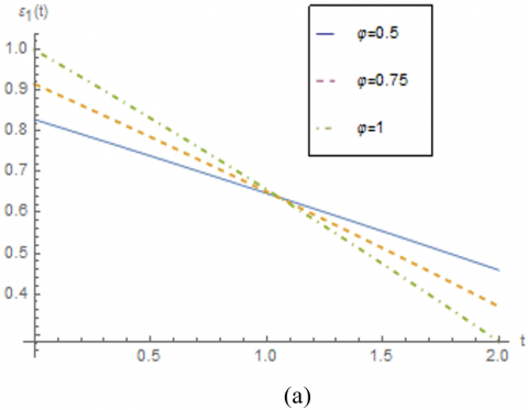
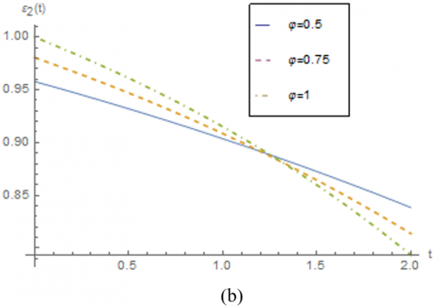
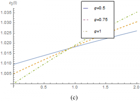
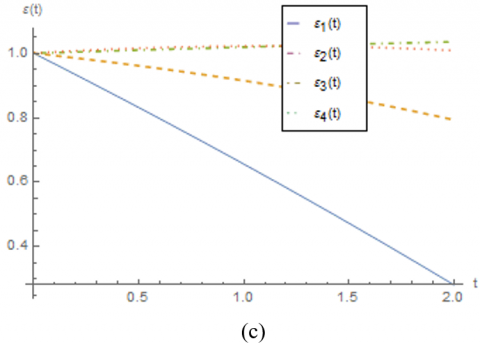
Figure 1. The response of the solutions (a) ε1(t), (b) ε2(t), (c) ε3(t) and (d) ε4(t) with respect to t for φ=0.5, 0.75, 1
Also, the approximate solutions for φ=0.5, 0.75, 1 are presented in Figure 1 at time [0, 2]. As mentioned before, ε1 is ERD of area A, ε2 is ERS of area B to A, ε3 is the ERI to area A and finally ε4 is the RER of area A. From Figure 1(a), we can observe that ERD for φ=0.5 it is decreased with time t and for φ=0.75 and 1 it is more decreased. In (b), ERS is almost in same condition with ERD. Based on (c), ERI to area A is increasing for φ=0.5 and it is more increasing for φ=0.75 and 1 and finally from (d) RER of area A for φ=0.5 is decreasing but for φ=0.75 and 1 and 0≤t≤1 is increasing and for 1≤t≤2 is decreasing.
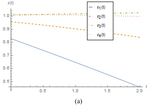
Figure 2, shows the approximate solutions of ε1(t), ε2(t), ε3(t) and ε4(t) for φ=0.5, 0.75, 1. From Figure 2, we can see that when ERD of area A is decreasing and ERS of area B to A is decreasing slowly then the ERI to area A is decreasing very slowly and the RER of area A is fix. The residual errors of ε1(t), ε2(t), ε3(t) and ε4(t) for φ=0.5, 0.75, 1 are presented in Table 1.
Figure 2. The plots of approximate solutions of ε1(t), ε2(t), ε3(t) and ε4(t) for (a) φ=0.5, (b) φ=0.75 and (c) φ=1
Table 1. The residual errors of ε1(t), ε2(t), ε3(t) and ε4(t) for φ=0.5, 0.75, 1
|
function |
t |
φ=0.5 |
φ=0.75 |
φ=1 |
|
ε1(t) |
0.0 |
0.147886 |
0.0709089 |
0 |
|
0.2 |
0.145562 |
0.0665751 |
0.00664704 |
|
|
0.4 |
0.143262 |
0.0622533 |
0.0133781 |
|
|
0.6 |
0.140988 |
0.0579496 |
0.0201769 |
|
|
0.8 |
0.138742 |
0.0536703 |
0.0270255 |
|
|
1.0 |
0.136526 |
0.0494219 |
0.0339046 |
|
|
1.2 |
0.13434 |
0.0452114 |
0.0407936 |
|
|
1.4 |
0.132186 |
0.041046 |
0.0476709 |
|
|
1.6 |
0.130066 |
0.0369329 |
0.054514 |
|
|
1.8 |
0.127981 |
0.0328796 |
0.0612996 |
|
|
2.0 |
0.125934 |
0.0288937 |
0.0680043 |
|
|
ε2(t) |
0.0 |
0.0224797 |
0.00859077 |
1.38778×10⁻¹⁷ |
|
0.2 |
0.0210296 |
0.00533641 |
0.00492826 |
|
|
0.4 |
0.0196747 |
0.00218032 |
0.00989604 |
|
|
0.6 |
0.0184181 |
0.000865924 |
0.0148763 |
|
|
0.7 |
0.0172635 |
0.00379033 |
0.01984 |
|
|
1.0 |
0.0162142 |
0.00658057 |
0.0247567 |
|
|
1.2 |
0.0152738 |
0.00922404 |
0.0295944 |
|
|
1.4 |
0.0144457 |
0.0117079 |
0.0343199 |
|
|
1.6 |
0.0137336 |
0.0140191 |
0.0388991 |
|
|
1.8 |
0.0131409 |
0.0161446 |
0.0432973 |
|
|
2.0 |
0.0126712 |
0.018071 |
0.0474794 |
|
|
ε3(t) |
0.0 |
0.00611767 |
0.00267734 |
0 |
|
0.2 |
0.00958746 |
0.00760386 |
0.0062537 |
|
|
0.4 |
0.0130939 |
0.0126045 |
0.0126191 |
|
|
0.6 |
0.0166373 |
0.017681 |
0.019102 |
|
|
0.7 |
0.020218 |
0.0228352 |
0.0257082 |
|
|
1.0 |
0.0238363 |
0.0280686 |
0.0324426 |
|
|
1.2 |
0.0274924 |
0.0333827 |
0.0393097 |
|
|
1.4 |
0.0311866 |
0.0387786 |
0.0463138 |
|
|
1.6 |
0.0349191 |
0.0442577 |
0.0534585 |
|
|
1.8 |
0.0386902 |
0.049821 |
0.0607473 |
|
|
2.0 |
0.0424999 |
0.0554695 |
0.0681831 |
|
|
ε4(t) |
0.0 |
0.020052 |
0.0144559 |
0 |
|
0.2 |
0.0182766 |
0.013136 |
1.05237×10⁻¹¹ |
|
|
0.4 |
0.0164984 |
0.0118146 |
3.40934×10⁻¹⁰ |
|
|
0.6 |
0.0147174 |
0.0104913 |
2.62041×10⁻⁹ |
|
|
0.7 |
0.0129333 |
0.00916531 |
1.11735×10⁻⁸ |
|
|
1.0 |
0.0111459 |
0.0078363 |
3.44944×10⁻⁸ |
|
|
1.2 |
0.00935498 |
0.00650376 |
8.68037×10⁻⁸ |
|
|
1.4 |
0.00756039 |
0.00516722 |
1.89681×10⁻⁷ |
|
|
1.6 |
0.00576193 |
0.00382627 |
3.73765×10⁻⁷ |
|
|
1.8 |
0.00395943 |
0.0024805 |
6.80508×10⁻⁷ |
|
|
2.0 |
0.00215273 |
0.00112953 |
1.16398×10⁻⁶ |
Based on the important role of functional calculus in different fields, we focused on the fractional model of nonlinear ES-DS. Using this applicable model we can adjust and control the supply and demand of the energy. Therefore, this model can be exploited for countries with limited energy resources. We applied the Caputo-Fabrizio derivative and its properties to solve the problem. Several theorems were proved to show the existence and uniqueness of solution and it is the main novelty of this study. We used the special data to forecast on the special time and based on them we found the numerical results. In the future researches, we will apply the fractional semi-analytical methods such as the homotopy analysis method and the homotopy perturbation method for solving the fractional model of ES-DS.
This work was supported by the base part of the Government Assignment for Scientific Research from the Ministry of Science and Higher Education of Russia (project code: 0667-2020-0039).
[1] Yuzbasi, S., Karacayr, M. (2017). An exponential galerkin method for solutions of HIV infection model of CD4+ T-cells. Computational Biology and Chemistry, 67: 205-212. http://dx.doi.org/10.1016/j.compbiolchem.2016.12.006
[2] Yuzbasi, S. (2012). A numerical approach to solve the model for HIV infection of CD4+T cells. Applied Mathematical Modelling, 36(12): 5876-5890. https://doi.org/10.1016/j.apm.2011.12.021
[3] Noeiaghdam, S., Khoshrouye Ghiasi, E. (2019). An efficient method to solve the mathematical model of HIV infection for CD8+ T-cells. International Journal of Mathematical Modelling & Computations, 9(4): 267-281.
[4] Noeiaghdam, S., Khoshrouye Ghiasi, E. (2019). Solving a non-linear model of HIV infection for CD4+ T cells by combining Laplace transformation and Homotopy analysis method. arXiv:1809.06232.
[5] Naik, P.A., Zu, J., Owolabi, K.M. (2020). Modeling the mechanics of viral kinetics under Immune Control during Primary Infection of HIV-1 with treatment in fractional order. Physica A: Statistical Mechanics and its Applications, 545: 1-19. http://dx.doi.org/10.1016/j.physa.2019.123816
[6] Naik, P.A., Zu, J., Owolabi, K.M. (2020). Global dynamics of a fractional order model for the Transmission of HIV Epidemic with Optimal Control. Chaos, Solitons & Fractals, 138: 1-24. https://doi.org/10.1016/j.chaos.2020.109826
[7] Naik, P.A. (2020). Global Dynamics of a fractional order SIR epidemic model with memory. International Journal of Biomathematics, 13(5): 1-20. https://doi.org/10.1142/S1793524520500710
[8] Ozturk, Y., Gulsu, M. (2015). Numerical solution of a modified epidemiological model for computer viruses. Applied Mathematical Modelling, 39(23-24): 7600-7610. https://doi.org/10.1016/j.apm.2015.03.023
[9] Singh, J., Kumar, D., Hammouch, Z., Atangana, A. (2018). A fractional epidemiological model for computer viruses pertaining to a new fractional derivative. Applied Mathematics and Computation, 316: 504-515. http://dx.doi.org/10.1016/j.amc.2017.08.048
[10] Noeiaghdam, S. (2019). Numerical approximation of modified non-linear SIR model of computer viruses. Contemporary Mathematics, 1(1): 34-48. http://dx.doi.org/10.37256/cm.11201959.34-48
[11] Noeiaghdam, S. (2019). A novel technique to solve the modified epidemiological model of computer viruses. SeMA Journal, 76(1): 97-108. http://dx.doi.org/10.1007/s40324-018-0163-3
[12] Noeiaghdam, S., Suleman, M., Budak, H. (2018). Solving a modified nonlinear epidemiological model of computer viruses by homotopy analysis method. Mathematical Sciences, 12(3): 211-222. http://dx.doi.org/10.1007/s40096-018-0261-5
[13] Guerrero, F., Santonja, F.J., Villanueva, R.J. (2013). Solving a model for the evolution of smoking habit in Spain with homotopy analysis method. Nonlinear Analysis: Real World Applications, 14(1): 549-558. https://doi.org/10.1016/j.nonrwa.2012.07.015
[14] Sikander, W., Khan, U., Ahmed, N., Mohyud-Din, S.T. (2017). Optimal solutions for a bio mathematical model for the evolution of smoking habit. Results in Physics, 7: 510-517. http://dx.doi.org/10.1016/j.rinp.2017.01.001
[15] Altaf Khan, M., Ullah, S., Farooq, M. (2018). A new fractional model for tuberculosis with relapse via Atangana–Baleanu derivative. Chaos, Solitons & Fractals, 116: 227-238. https://doi.org/10.1016/j.chaos.2018.09.039
[16] Sweilam, N.H., AL-Mekhlafi, S.M. (2016). Numerical study for multi-strain tuberculosis (TB) model of variable-order fractional derivatives. Journal of Advanced Research, 7(2): 271-283. http://dx.doi.org/10.1016/j.jare.2015.06.004
[17] Günerhan, H., Dutta, H., Weaver, M.A., Adel, W. (2020). Analysis of a fractional HIV model with Caputo and constant proportional Caputo operators. Chaos, Solitons & Fractals, 139: 110053. https://doi.org/10.1016/j.chaos.2020.110053
[18] Guerrero Sánchez, Y., Sabir, Z., Günerhan, H., Baskonus, H.M. (2020). Analytical and approximate solutions of a novel nervous stomach mathematical model. Discrete Dynamics in Nature and Society, 2020: 5063271. https://doi.org/10.1155/2020/5063271
[19] Ghanbari, B., Günerhan, H., Srivastava, H.M. (2020). An application of the Atangana-Baleanu fractional derivative in mathematical biology: A three-species predator-prey model. Chaos, Solitons & Fractals, 138: 109910. https://doi.org/10.1016/j.chaos.2020.109910
[20] Srivastava, H.M., Günerhan, H. (2019). Analytical and approximate solutions of fractional-order susceptible-infected-recovered epidemic model of childhood disease. Mathematical Methods in the Applied Sciences, 42(3): 935-941. http://dx.doi.org/10.1002/mma.5396
[21] Sun, M., Tian, L., Xu, J. (2006). Time-delayed feedback control of the energy resource chaotic system. International Journal of Nonlinear Science, 1(3): 172-177.
[22] Sun, M., Tian, L. (2007). An energy resources demand-supply system and its dynamical analysis. Chaos, Solitons & Fractals, 32(1): 168-180. http://dx.doi.org/10.1016/j.chaos.2005.10.085
[23] Sun, M., Tian, L.X., Jia, Q. (2009). Adaptive control and synchronization of a four-dimensional energy resources system with unknown parameters. Chaos Solitons Fract, 39(4): 1943-1949. http://dx.doi.org/10.1016/j.chaos.2007.06.117
[24] Sun, M., Tao, Y., Wang, X., Tian, L. (2011). The model reference control for the four-dimensional energy supply-demand system. Applied Mathematical Modelling, 35(10): 5165-5172. http://dx.doi.org/10.1016/j.apm.2011.04.016
[25] Sun, M., Jia, Q., Tian, L. (2009). A new four-dimensional energy resources system and its linear feedback control. Chaos, Solitons & Fractals, 39(1): 101-108. http://dx.doi.org/10.1016/j.chaos.2007.01.125
[26] Sidorov, D., Muftahov, I., Tomin, N., Karamov, D., Panasetsky, D., Dreglea, A., Liu, F., Foley, A. (2020). A dynamic analysis of energy storage with renewable and diesel generation using volterra equations. IEEE Transactions on Industrial Informatics, 16(5): 3451-3459. https://doi.org/10.1109/TII.2019.2932453
[27] Wang, Q., Ma, J., Yu, S., Tan, L. (2020). Noise detection and image denoising based on fractional calculus. Chaos, Solitons & Fractals, 131: 109463. http://dx.doi.org/10.1016/j.chaos.2019.109463
[28] Chen, T., Wang, D. (2020). Combined application of blockchain technology in fractional calculus model of supply chain financial system. Chaos, Solitons & Fractals, 131: 109461. https://doi.org/10.1016/j.chaos.2019.109461
[29] Zhang, Q., Cui, N., Li, Y., Duan, B., Zhang, C. (2020). Fractional calculus based modeling of open circuit voltage of lithium-ion batteries for electric vehicles. Journal of Energy Storage, 27: 100945. http://dx.doi.org/10.1016/j.est.2019.100945
[30] Angelis, P.D., Marchis, R.D., Martire, A.L., Oliva, I. (2020). A mean-value Approach to solve fractional differential and integral equations. Chaos, Solitons & Fractals, 138: 109895. https://doi.org/10.1016/j.chaos.2020.109895
[31] Odibat, Z. (2006). Approximations of fractional integrals and Caputo fractional derivatives. Applied Mathematics and Computation, 178(2): 527-533. http://dx.doi.org/10.1016/j.amc.2005.11.072
[32] Jahanshahi, S., Babolian, E., Torres, D.F.M., Vahidi, A.R. (2017). A fractional Gauss–Jacobi quadrature rule for approximating fractional integrals and derivatives. Chaos, Solitons & Fractals, 102: 295-304. https://doi.org/10.1016/j.chaos.2017.04.034
[33] Suleman, M., Lu, D., He, J.H., Farooq, U., Noeiaghdam, S., Chandio, F.A. (2018). Elzaki projected differential transform method for fractional order system of linear and nonlinear fractional partial differential equation. Fractals, 36(3): 1850041. http://dx.doi.org/10.1142/S0218348X1850041X
[34] Caputo, M., Fabrizio, M. (2015). A new definition of fractional derivative without singular Kernel. Progr. Fract. Differ. Appl., 1: 73-85. http://dx.doi.org/10.12785/pfda/010201
[35] Losada, J., Nieto, J.J. (2015). Properties of the new fractional derivative without singular Kernel. Progr. Fract. Differ. Appl., 1: 87-92. http://dx.doi.org/10.12785/pfda/010202