Sharmin Sultana Shanta* | Md. Azmir Ibne Islam | Kamonashis Mondol | Sarder Firoz Ahmmed
© 2020 IIETA. This article is published by IIETA and is licensed under the CC BY 4.0 license (http://creativecommons.org/licenses/by/4.0/).
OPEN ACCESS
Present study is devoted for an unsteady flow mass and heat transfer past a vertical porous plate with variable viscosity. The effects of chemical reaction, heat source and thermal conductivity on the flow are also investigated. The partial differential equations, which are essentially nonlinear in nature, along with specific boundary conditions have been converted to the dimensionless form by using appropriate coordinate transformation. Explicit finite difference method has been applied to solve the dimensionless momentum, concentration and energy equations numerically. The velocity, concentration and temperature outlines have been discussed for well-known parameters whereas Nusselt number and skin friction have been represented in tabular forms. The variations of stream lines and isotherms have also been displayed graphically. Absolute conclusion has finally been drawn based on the numerical and graphical results.
explicit finite difference method, mass transfer, unsteady flow, variable viscosity, vertical porous plate
In numerous significant fields like chemical engineering, industrial areas and geophysical sciences, the knowledge of mass and heat transfer flow is very essential. Unsteady flows continuously play a vital part in aerospace technologies and turbo-machineries. Researchers throughout the recent decades have performed several experiments. As a result, remarkable findings have been seen to reveal. For example, Ahmed et al. [1] investigated the MHD periodic flow past an isothermal oscillating cylinder and observed the effects of thermal conductivity and temperature dependent viscosity. An incompressible fluid flow, in a porous medium, of mass and heat transfer with viscous dissipation and suction along with hall effect has been inspected by Ali et al. [2]. The chemically reactive fluid flow examined by Arifuzzaman et al. [3] revealed the absorption radiation effect in the existence of oscillatory vertical plate. The unsteady mass and heat transfer MHD flow convection has been discussed by Aurangzaib et al. [4] in the appearance of a saturated medium with micro polar fluid. Simulation of magneto hydrodynamic forced convective boundary layer flow has been studied by Devi et al. [5] by adopting Nachtsheim Swigert shooting and fourth order Runge Kutta methods, from where it has been revealed that the heat and flow transfer characteristics altered for the existence or presence of magnetic field and heat source. Ghara et al. [6] worked on MHD free convection flow with ramped wall temperature and observed the effect of radiation while the fluid was passing through a moving vertical plate. Hayat et al. [7] considered Casson nanofluid, inspected the mixed convention flow and examined the heat sink/source together with chemical reaction along a stretching sheet. A mathematical simulation was done by Hossain et al. [8] on unsteady flow convection over a vertically isothermal cylinder by means of viscosity which was dependent on temperature. They considered a cylinder which was vertically semi-infinite, used explicit finite difference method and examined air convective free flow to explore the viscosity properties. The unsteady free convection flow of incompressible viscous fluid with Newtonian heating and mass diffusion past a vertical plate has been analyzed by Hussanan et al. [9] with the help of Laplace Transforms. Karthikeyan et al. [10] used perturbation technique in order to study the MHD flow with radiation thermal effects through a plate in porous medium. Chebyshev spectral method has been used by Khader et al. [11] to establish the approximate solution of a Newtonian fluid which was electrically charged through an impermeable extending sheet. Makanda et al. [12] studied the casson fluid considering magnetic field effect in porous medium. Runge Kutta Fehlberg integration and successive linearization methods have been used for investigating the effect of different parameters. Mondal et al. [13] investigated the flow of casson fluid for thermal conductivity and variable viscosity. The effects of heat source along with viscous dissipation on unsteady MHD flow through a sheet, which is stretching, have been reflected in the work of Reddy et al. [14] where Keller Box method has been used to examine the heat source and viscous dissipation. Rehman et al. [15] showed the consequences of thermal stratification and thermal radiations on hyperbolic tangent fluid flow produced by cylindrical and flat surfaces. Veeresh et al. [16] explored the consequences of viscous dissipation, Joule heating and temperature heat source properties on magneto hydrodynamic free convection, chemically reactive and radiative flow by using perturbation technique.
Unsteady flow through an infinite vertical plate was explored by Uwanta et al. [17]. Crank-Nicolson method was used to analyze the mass and heat transfer with the existence of thermal conductivity, chemical reaction and heat source parameter. Keeping all these thoughts in mind, we are fully motivated to focus on the effort done by Uwanta et al. [17] and want to examine the velocity, concentration and temperature outlines with variable viscosity. In other words, the objectives of this present research are to observe the effects of unsteady flow mass and heat transfer through a vertical porous plate along with thermal conductivity, chemical reaction, heat source and variable viscosity parameters. We are determined to apply an explicit finite difference method in order to obtain the numerical solutions of the governing equations. To be more specific, the problem formulation has been represented in Section 2. The numerical technique to solve the dimensionless equations is discussed in Section 3. In Section 4, numerical simulations with physical significance are reported graphically and the effects of various factors on velocity, concentration and temperature outlines are reflected. Moreover, the stream lines and isotherms have been displayed graphically whereas Nusselt number and skin friction have been demonstrated in tabular format. Section 5 finally contains the whole summary of our investigation.
A two dimensional unsteady natural laminar convective flow of incompressible viscous, dissipative and radiating fluid (water or air) is considered along an isothermal infinite vertical porous plate. The acceleration due to the gravity (g) is assumed to be acted in downward direction. The $\bar{x}$-axis is considered to be directed upward along the vertical porous plate whereas $\bar{y}$-axis is always normal to the plate. We assume that the fluid and the plate are initially (i.e., at time$\bar{t}=0$) held at the similar temperature (${{\bar{T}}_{\infty }}$) and species concentration (${{\bar{C}}_{\infty }}$). The fluid starts moving along the vertical porous plate at $\bar{t}>0$, consequently, the temperature of the plate and the species concentration are elevated to ${{\bar{T}}_{w}}$ and ${{\bar{C}}_{w}}$ respectively which cause the differences both in temperature (${{\bar{T}}_{w}}-{{\bar{T}}_{\infty }}$) and in concentration (${{\bar{C}}_{w}}-{{\bar{C}}_{\infty }}$). Since the plate, in extent, is infinite, the physical variables are actually independent of $\bar{x}$ and are the functions of $\bar{t}\,$and$\bar{y}$. The variable viscosity, the nth-order chemical reaction and the variable thermal conductivity are assumed to be non-constant. It is also assumed that the thermal radiation is actually present as a form of a uni-directional flux along$\bar{y}$direction which means that the radiative heat flux (qr) is principally transverse with the vertical surface and can be expressed under Rosseland approximation as:
$\frac{\partial {{q}_{r}}}{\partial \overline{y}}=-\,4\sigma \,{{a}^{*}}\left( \overline{T}_{\infty }^{4}-{{\overline{T}}^{4}} \right)$
where, a* denotes the mean absorption effect for the thermal radiation constant, σ represents the Stefan-Boltzmann constant. It is our assumption that the differences in temperature within the flow are small enough, therefore we can expand ${{\overline{T}}^{4}}$in Taylor series about ${{\overline{T}}_{\infty }}$by neglecting the higher order terms as ${{\overline{T}}^{4}}\cong 4\overline{T}\overline{T}_{\infty }^{3}-3\overline{T}_{\infty }^{4}$.
Keeping Boussinesq approximation in mind, the governing equations such as continuity, momentum, concentration and energy along the velocity components $\bar{u}$ and $\bar{v}$ at $\bar{t}$in $\bar{x}$ and$\bar{y}$directions can be written as:
$\frac{\partial \overline{v}}{\partial \overline{y}}=0$ (1)
$\begin{align} & \frac{\partial \overline{u}}{\partial \overline{t\,}}+\overline{v}\frac{\partial \overline{u}}{\partial \overline{y}}=\frac{1}{\rho }\frac{\partial }{\partial \overline{y}}\left( \mu \,(\overline{T})\frac{\partial \overline{u}}{\partial \overline{y}} \right)-\frac{\sigma {{B}_{\circ }}^{2}\overline{u}}{\rho }-\frac{\upsilon \overline{u}}{{{K}^{*}}} \\ & \,\,\,\,\,\,\,\,\,\,\,\,\,\,\,\,\,\,\,\,\,\,+g\beta (\overline{T}-{{\overline{T}}_{\infty }})+g{{\beta }^{*}}(\overline{C}-{{\overline{C}}_{\infty }})-b_{1}^{*}{{\overline{u}}^{2}} \\ \end{align}$ (2)
$\frac{\partial \overline{C}}{\partial \overline{t\,}}+\overline{v}\frac{\partial \overline{C}}{\partial \overline{y}}=D\frac{{{\partial }^{2}}\overline{C}}{\partial {{\overline{y}}^{2}}}-{{R}^{*}}{{(\overline{C}-{{\overline{C}}_{\infty }})}^{n}}$ (3)
$\begin{align} & \frac{\partial \overline{T}}{\partial \overline{t\,}}+\overline{v}\frac{\partial \overline{T}}{\partial \overline{y}}=\frac{1}{\rho \,{{C}_{p}}}\frac{\partial }{\partial \overline{y}}\left( K(\overline{T})\frac{\partial \overline{T}}{\partial \overline{y}} \right)-\frac{1}{\rho {{C}_{p}}}\frac{\partial {{q}_{r}}}{\partial \overline{y}} \\ & \,\,\,\,\,\,\,\,\,\,\,\,\,\,\,\,\,\,\,\,\,\,\,\,\,\,+\frac{\upsilon }{{{C}_{p}}}{{\left( \frac{\partial \overline{u}}{\partial \overline{y}} \right)}^{2}}+{{b}^{*}}{{\overline{u}}^{2}}+\frac{Q}{\rho \,{{C}_{p}}}(\,\overline{T}-{{\overline{T}}_{\infty }}) \\ \end{align}$ (4)
with the corresponding boundary conditions:
$\left. \begin{align} & \overline{t\,}\le 0,\,\,\,\,\,\,\overline{u}=0,\,\,\,\overline{T}={{\overline{T}}_{\infty }},\,\,\,\overline{C}={{\overline{C}}_{\infty }}\,\,\,\,\,\,\,\,\,\,\text{for}\,\,\text{all}\,\,\,\overline{y} \\ & \overline{t\,}\,\,>0,\,\,\,\,\,\,\overline{u}=0,\,\,\,\overline{T}={{\overline{T}}_{w}},\,\,\,\overline{C}={{\overline{C}}_{w}}\,\,\,\,\,\,\,\,\,\,\text{at}\,\,\,\,\overline{y}=0\,\,\,\,\,\, \\ & \,\,\,\,\,\,\,\,\,\,\,\,\,\,\,\,\,\,\overline{u}\to 0,\,\,\overline{T}\to \,{{\overline{T}}_{\infty }},\,\,\overline{C}\to \,{{\overline{C}}_{\infty }}\,\,\,\,\,\,\,\text{as}\,\,\,\overline{y}\to \infty \\ \end{align} \right\}\,$ (5)
From Eq. (1), we understand that suction velocity may take the form of a constant or a function of time. By integrating Eq. (1), suction velocity is assumed as $\overline{v}=-\,{{v}_{0}}$which is perpendicular to the plate where v0 represents the scale of suction velocity. Here, negative sign specifies the phenomena that suction is in the direction of the plate. Also, ${{v}_{0}}>0$is corresponding to the steady suction velocity perpendicular to the surface.
Now we apply the following dimensionless quantities:
$\begin{align} & U=\frac{\overline{u}}{{{U}_{\circ }}},\,\,\,y=\frac{\overline{y}\,{{U}_{\circ }}}{\upsilon },\,\,\,t=\frac{\overline{t\,}\,{{U}_{\circ }}^{2}}{\upsilon },\,\,\,\, \\ & \theta =\frac{\overline{T}-{{\overline{T}}_{\infty }}}{{{\overline{T}}_{w}}-{{\overline{T}}_{\infty }}},\,\,\,C=\frac{\overline{C}-{{\overline{C}}_{\infty }}}{{{\overline{C}}_{w}}-{{\overline{C}}_{\infty }}},\,\,\,\,b=\frac{{{b}^{*}}\upsilon }{{{\overline{T}}_{w}}-{{\overline{T}}_{\infty }}},\,\,\,\, \\ & Sc=\frac{\upsilon }{D},\,\,\,M=\frac{\upsilon \sigma B_{\circ }^{2}}{\rho U_{\circ }^{2}},\,\,\,\alpha =\frac{{{\upsilon }_{\circ }}}{{{U}_{\circ }}},\,\,\,{{b}_{1}}=\frac{b_{1}^{*}\upsilon }{{{U}_{\circ }}},\,\, \\ & K=\frac{{{K}^{*}}U_{\circ }^{2}}{{{\upsilon }^{2}}},\,\,\,\,N=\frac{16{{a}^{*}}\sigma \overline{T}_{\infty }^{3}{{\upsilon }^{2}}}{{{k}_{\circ }}{{U}_{\circ }}^{2}},\,\,\,\Pr =\frac{\upsilon \rho {{C}_{p}}}{{{k}_{\circ }}},\,\,\,\, \\ & Ec=\frac{U_{\circ }^{2}}{{{C}_{p}}({{\overline{T}}_{w}}-{{\overline{T}}_{\infty }})},\,\,\,\,Gr=\frac{g\beta \upsilon \,({{\overline{T}}_{w}}-{{\overline{T}}_{\infty }})}{U_{\circ }^{3}},\,\,\, \\ & Gc=\frac{g{{\beta }^{*}}\upsilon \,({{\overline{C}}_{w}}-{{\overline{C}}_{\infty }})}{U_{\circ }^{3}},\,\,\upsilon =\frac{{{\mu }_{0}}}{\rho } \\ \end{align}$ (6)
We now use the dimensional variable thermal conductivity:
$K(\overline{T})={{k}_{\text{o}}}(1+{{\gamma }_{10}}(\,\overline{T}-{{\overline{T}}_{\infty }})\,)$
which depends on the temperature. Here, γ10 is any constant and ko is the thermal conductivity of ambient fluid. Let τ be the dimensionless variable thermal conductivity which can be written as$\,\tau ={{\gamma }_{10}}({{\overline{T}}_{w}}-{{\overline{T}}_{\infty }})$. Therefore, $K(\overline{T})={{k}_{\text{o}}}(1+\tau \theta \,)$.
We also incorporate the dimensional variable viscosity:
$\mu \,(\overline{T})={{\mu }_{\text{o}}}(1+{{\gamma }_{20}}(\,\overline{T}-{{\overline{T}}_{\infty }})\,)$
Here, γ20 is any constant and μo is the variable viscosity of ambient fluid. Let γ is the dimensionless variable viscosity which may be defined as $\gamma ={{\gamma }_{20}}(\,{{\overline{T}}_{w}}-{{\overline{T}}_{\infty }})$.
Therefore, $\mu \,(\overline{T})={{\mu }_{0}}\,(\,1+\gamma \,\theta \,)$.
We also take into account the dimensionless chemical reaction parameter:
$Kr=\frac{\upsilon {{R}^{*}}{{({{\overline{C}}_{w}}-{{\overline{C}}_{\infty }})}^{n-1}}}{U_{\circ }^{2}}$
where, R* is representing the dimensional chemical reaction and n is denoting the reaction order.
A dimensionless heat source parameter S to provide the temperature is introduced as:
$S=\frac{Q{{\upsilon }^{2}}}{{{k}_{\circ }}{{U}_{\circ }}^{2}}\,$
where, Q denotes the volumetric rate of heat source.
Finally by applying the dimensionless quantities, Eqns. (1)-(4) reduce to:
$\begin{align} & \left( \frac{\partial U}{\partial t}-\alpha \frac{\partial U}{\partial y} \right)=(1+\gamma \,\theta )\frac{{{\partial }^{2}}U}{\partial {{y}^{2}}}+\gamma \,\left( \frac{\partial \theta }{\partial y} \right)\,\left( \frac{\partial U}{\partial y} \right) \\ & \,\,\,\,\,\,\,\,\,\,\,\,\,\,\,\,\,\,\,\,\,\,\,\,\,\,\,\,\,\,\,\,\,\,-\left( M-\frac{1}{k} \right)U+Gr\theta +GcC-{{b}_{1}}{{U}^{2}} \\ \end{align}$ (7)
$\frac{\partial C}{\partial t}-\alpha \frac{\partial C}{\partial y}=\frac{1}{Sc}\frac{{{\partial }^{2}}C}{\partial {{y}^{2}}}-Kr{{C}^{n}}$ (8)
$\begin{align} & \frac{\partial \theta }{\partial t}-\alpha \frac{\partial \theta }{\partial y}=\frac{(1+\tau \theta )}{\Pr }\frac{{{\partial }^{2}}\theta }{\partial {{y}^{2}}}+{{\left( \frac{\partial \theta }{\partial y} \right)}^{2}}\frac{\tau }{\Pr } \\ & \,\,\,\,\,\,\,\,\,\,\,\,\,\,\,\,\,\,\,\,\,\,\,\,\,\,\,\,\,\,\,\,\,\,\,\,\,\,\,\,+\frac{\left( S-N \right)}{\Pr }\theta +Ec\,{{\left( \frac{\partial U}{\partial y} \right)}^{2}}+b{{U}^{2}} \\ \end{align}$ (9)
The boundary conditions for the problem are given below:
$\left. \begin{align} & \,t\le 0,\,\,\,\,\,\,\,\,U=0,\,\,\,\theta =0,\,\,\,C=0\,\,\,\,\,\,\,\,\,\,\,\,\,\,\text{for}\,\,\text{all}\,\,y\,\,\,\,\, \\ & \,t>0,\,\,\,\,\,\,\,\,U=0,\,\,\,\theta =1,\,\,\,C=1\,\,\,\,\,\,\,\,\,\,\,\,\,\,\,\,at\,\,y=0\,\, \\ & \,\,\,\,\,\,\,\,\,\,\,\,\,\,\,\,\,\,\,\,U\to 0,\,\,\,\theta \to 0,\,\,\,C\to 0\,\,\,\,\,\,\,as\,\,y\to \infty \\ \end{align} \right\}$ (10)
The physical quantities, i.e., Nusselt number (Nu) and skin friction (Cf ) can be written in dimensionless form as follows:
$Nu=\frac{1}{\sqrt{2}}G{{r}^{-\,\frac{3}{4}}}{{\left( \frac{\partial \theta }{\partial y} \right)}_{y=0}}$ and ${{C}_{f}}=-\frac{1}{2\sqrt{2}}G{{r}^{-\,\frac{3}{4}}}{{\left( \frac{\partial U}{\partial y} \right)}_{y=0}}$
Explicit finite difference method has been applied to obtain the solution of the Eqns. (7)-(9) with boundary conditions Eq. (10). The boundary layer area is subdivided by perpendicular lines generated from y-axis. Figure 1 displays the grid space by considering the maximum height of the plate: xmax = 20, maximum height of the boundary layer: ymax= 50, grid spacing: m1 = 100, n1 = 200 with ∆x = 0.20 (0 ≤ x ≤ 20) and ∆y = 0.25 (0 ≤ y ≤ 50). A small time step ∆t is taken as 0.005.
Figure 1. Grid space based on finite difference
Now we define U, C and θ in the finite difference form:
${{\left( \frac{\partial U}{\partial t} \right)}_{i,\,\,j}}=\frac{{{U}_{new}}-U_{i,\,\,j}^{{}}}{\Delta t},$
${{\left( \frac{{{\partial }^{2}}U}{\partial {{y}^{2}}} \right)}_{i,\,\,j}}=\frac{{{U}_{i,\,\,j+1}}+{{U}_{i,\,\,j-1}}-2{{U}_{i,\,\,j}}}{{{(\Delta y)}^{2}}},$
${{\left( \frac{\partial C}{\partial t} \right)}_{i,\,\,j}}=\frac{{{C}_{new}}-C_{i,\,\,j}^{{}}}{\Delta t},$ ${{\left( \frac{\partial C}{\partial y} \right)}_{i,\,\,j}}=\frac{C_{i,\,\,j+1}^{{}}-C_{i,\,\,j}^{{}}}{\Delta y},$
${{\left( \frac{{{\partial }^{2}}C}{\partial {{y}^{2}}} \right)}_{i,\,\,j}}=\frac{{{C}_{i,\,\,j+1}}+{{C}_{i,\,\,j-1}}-2{{C}_{i,\,\,j}}}{{{(\Delta y)}^{2}}},$
${{\left( \frac{\partial \theta }{\partial t} \right)}_{i,\,\,j}}=\frac{{{\theta }_{new}}-\theta _{i,\,\,j}^{{}}}{\Delta t},$ ${{\left( \frac{\partial \theta }{\partial y} \right)}_{i,\,\,j}}=\frac{\theta _{i,\,\,j+1}^{{}}-\theta _{i,\,\,j}^{{}}}{\Delta y},$
${{\left( \frac{{{\partial }^{2}}\theta }{\partial {{y}^{2}}} \right)}_{i,\,\,j}}=\frac{{{\theta }_{i,\,\,j+1}}+{{\theta }_{i,\,\,j-1}}-2{{\theta }_{i,\,\,j}}}{{{(\Delta y)}^{2}}}.$
Using the above forms in Eqns. (7)-(10), we get a suitable set of equations as:
$\begin{align} & \frac{{{U}_{new}}-U_{i,\,\,j}^{{}}}{\Delta t}-\alpha \frac{U_{i,\,\,j+1}^{{}}-U_{i,\,\,j}^{{}}}{\Delta y} \\ & \,\,\,\,\,\,\,\,\,\,\,\,\,=(1+\gamma \,\theta _{i\,,\,j}^{{}})\frac{{{U}_{i,\,\,j+1}}+{{U}_{i,\,\,j-1}}-2{{U}_{i,\,\,j}}}{{{(\Delta y)}^{2}}}\, \\ & \,\,\,\,\,\,\,\,\,\,\,\,\,\,\,\,\,\,\,\,+\gamma \,\frac{\theta _{i,\,\,j+1}^{{}}-\theta _{i,\,\,j}^{{}}}{\Delta y}\frac{U_{i,\,\,j+1}^{{}}-U_{i,\,\,j}^{{}}}{\Delta y}\,-\left( M-\frac{1}{k} \right)U_{i,\,\,j}^{{}} \\ & \,\,\,\,\,\,\,\,\,\,\,\,\,\,\,\,\,\,\,\,\,\,\,\,\,\,\,\,\,\,\,\,\,\,\,\,\,\,\,\,\,\,\,\,\,\,\,\,\,+Gr\theta _{i,\,\,j}^{{}}+GcC_{i,\,\,j}^{{}}-{{b}_{1}}{{(U_{i,\,\,j}^{{}})}^{2}} \\ \end{align}$ (11)
$\begin{align} & \frac{{{C}_{new}}-C_{i,\,\,j}^{{}}}{\Delta t}-\alpha \frac{C_{i,\,\,j+1}^{{}}-C_{i,\,\,j}^{{}}}{\Delta y} \\ & \,\,\,\,\,\,\,\,\,\,\,\,\,\,\,\,\,\,\,=\frac{1}{Sc}\frac{{{C}_{i,\,\,j+1}}+{{C}_{i,\,\,j-1}}-2{{C}_{i,\,\,j}}}{{{(\Delta y)}^{2}}}-Kr{{(C_{i,\,\,j}^{{}})}^{n}} \\ \end{align}$ (12)
$\begin{align} & \frac{{{\theta }_{new}}-\theta _{i,\,\,j}^{{}}}{\Delta t}-\alpha \frac{\theta _{i,\,\,j+1}^{{}}-\theta _{i,\,\,j}^{{}}}{\Delta y} \\ & =\frac{(\tau \,\theta _{i\,,\,j}^{{}}+1)}{\Pr }\frac{{{\theta }_{i,\,\,j+1}}+{{\theta }_{i,\,\,j-1}}-2{{\theta }_{i,\,\,j}}}{{{(\Delta y)}^{2}}}+{{\left( \frac{\theta _{i,\,\,j+1}^{{}}-\theta _{i,\,\,j}^{{}}}{\Delta y} \right)}^{2}}\frac{\tau }{\Pr } \\ & \,\,\,\,\,\,\,\,\,\,\,+\frac{(S-N)}{\Pr }\theta _{i,\,\,j}^{{}}+Ec\,{{\left( \frac{U_{i,\,\,j+1}^{{}}-U_{i,\,\,j}^{{}}}{\Delta y} \right)}^{2}}+b{{(U_{i,\,\,j}^{{}})}^{2}} \\ \end{align}$ (13)
subject to the boundary conditions:
$\left. \begin{align} & \,t>0,\,\,\,\,U_{i\,,\,j}^{0}=0,\,\,\theta _{i\,,\,j}^{0}=1,\,\,C_{i\,,\,j}^{0}=1\,\,\,\,\,\,\,\,\,\,\,when\,\,y=0\,\,\, \\ & \,\,\,\,\,\,\,\,\,\,\,\,\,\,\,U_{i\,,\,j}^{n}\to 0,\,\,\theta _{i\,,\,j}^{n}\to 0,\,\,C_{i\,,\,j}^{n}\to 0\,\,\,\,when\,\,y\to \infty \, \\ \end{align} \right\}\,$ (14)
The dimensionless velocity, concentration and temperature outlines are discussed numerically with governing parameters: thermal Grashof number (Gr), mass Grashof number (Gc), suction parameter (α), variable thermal conductivity (τ), variable viscosity parameter (γ), inertia number (b1), hall current parameter (b), chemical reaction parameter (Kr), porosity (K), magnetic field parameter (M), Schmidt number (Sc), heat source parameter (S), Prandtl number (Pr), Eckert number (Ec) and finally thermal radiation parameter (N). The constant values of these parameters have been provided in Table 1. The variations of velocity outlines have been shown from Figures 2-8. Temperature outlines are represented from Figures 9-13 whereas Figures 14-16 represent the concentration outlines. Stream lines along with isotherms have been plotted and represented in Figures 17-20.
Table 1. Constant values of the parameters
|
Parameters |
Gr |
Gc |
α |
τ |
γ |
b1 |
b |
Kr |
|
Values |
1.0 |
1.0 |
3.0 |
0.1 |
0.25 |
1.0 |
1.0 |
0.1 |
|
Parameters |
K |
M |
Sc |
S |
Pr |
Ec |
N |
|
|
Values |
0.1 |
1.0 |
0.22 |
0.1 |
1.0 |
0.01 |
1.0 |
|
Figure 2 displays the velocity outlines for variable viscosity parameter (γ). Since viscosity is responsible for flow resistance, we see that velocity decreases when viscosity increases. Velocity peaks decrease about 3.33%, 6.67% and 7.33% when γ is changed from its base value 0.25 to 0.50, 0.75 and 1.0 respectively.
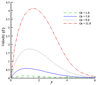
Figure 3 represents that velocity outlines decrease significantly with the increase of suction parameter (α). When α changes from 3.0 to 5.0, velocity peak declines about 35.53%. Similarly, peak value declines near about 52.63% (when α = 7.0) and 63.16% (when α = 9.0) compared to the peak value found for the baseline of α. From Figure 4, it has been observed that velocity outlines increase with the increase of thermal Grashof number (Gr).
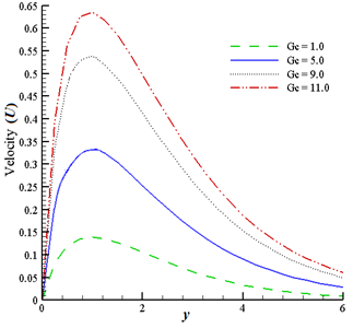
Figure 5 also shows the similar result, i.e., velocity outlines increase when the value of the mass Grashof number (Gc) is increased. We observe from Figure 6 that velocity outlines show declining effects when the inertia number (b1) is increased. Peak magnitudes decrease to 10.14%, 18.12% and 24.64% when b1 is increased from 1.0 to 15.0, 30.0 and 45.0 respectively. This phenomenon occurs, i.e., the velocity of the fluid tends to decrease, due to the air resistance and friction.
Figure 2. Velocity outlines for γ
Figure 3. Velocity outlines for α
Figure 4. Velocity outlines for Gr
Figure 5. Velocity outlines for Gc
Figure 6. Velocity outlines for b1
Figure 7. Velocity outlines for b
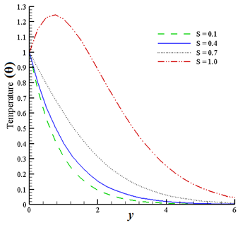
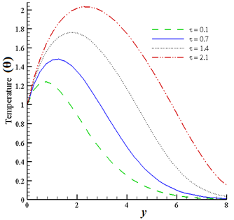
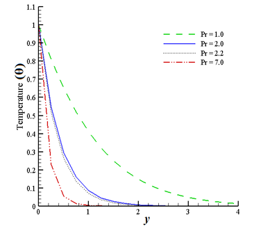
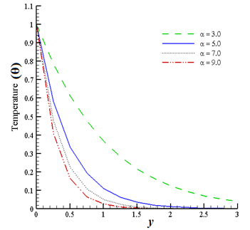
Figure 7 represents the velocity outlines with respect to the hall current parameter (b). We understand that velocity distributions rise to 5.07%, 12.32% and 23.18% with the increase of the parameter b from 1.0 to 5.0, 10.0 and 15.0 respectively. Due to the hall current, an electric field is experienced as a result of which, fluid velocity increases. From Figure 8, it is found that the velocity outlines decrease with the increase of the magnetic field parameter (M). This happens because larger values of M generate a drag force or Lorentz force which competes against the motion of the fluid. Figure 9 shows that the temperature outlines increase when the values of the heat source parameter (S) are increased (i.e., S = 0.1, 0.4, 0.7, 1.0). Temperature distribution for variable thermal conductivity (τ) is shown in Figure 10. We understand that compared to the baseline value of τ (i.e., τ = 0.1), temperature outlines increase about 16% (for τ = 0.7), 40% (for τ = 1.4) and 60% (for τ = 2.1). Variations in temperature outlines for multiple values of Prandtl number (Pr = 1.0, 2.0, 2.2, 7.0) have been represented in Figure 11, from where it has been perceived that temperature outlines decrease while Pr is increased. Similar result is seen from Figure 12 where the temperature distribution is represented for α = 3.0, 5.0, 7.0 and 9.0.
Figure 8. Velocity outlines for M
Figure 9. Temperature outlines for S
Figure 13 demonstrates the temperature outlines for thermal radiation parameter N = 1.0, 7.0, 14.0 and 21.0. We observe that temperature outlines decrease significantly when N is increased. From Figure 14, we notice that concentration outlines tend to decrease with the increase of chemical reaction parameter (Kr). Concentration outlines decrease to 25%, 79.31% and 89.66% when Kr is increased to 1.5, 15.0 and 25.0 respectively from its baseline value.
Figure 10. Temperature outlines for τ
Figure 11. Temperature outlines for Pr
Figure 12. Temperature outlines for α
Figure 13. Temperature outlines for N
Figure 14. Concentration outlines for Kr
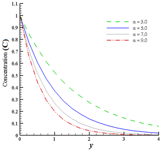
Figure 15. Concentration outlines for α
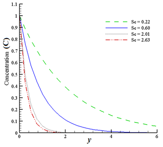
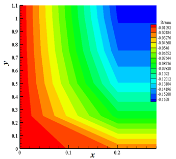
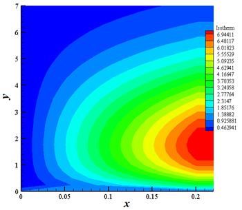
Figure 15 displays that concentration outlines decline due to the increase of α. Similar effects can be observed from Figure 16, that means, concentration outlines drop with the increase of Schmidt number (Sc). Figure 17 and Figure 18 represent the streamlines aimed at γ = 0.25 and γ = 0.50 respectively. We see that the streamlines increase with the increase of variable viscosity which has an effect on momentum along with thermal boundary layers. Isotherms are displayed in Figures 19-20 with respect to γ. It is revealed that isotherms show declining effects when γ is changed from 0.25 to 0.50. The variation of Nusselt number (Nu) has been shown in Table 2 for Gr, Gc, α, τ, γ, b1, b, Kr, K, M, Sc, S, Pr, Ec and N. It is observed that Nusselt number shows decreasing effect for Gr, Gc, τ, b, K and Ec whereas increasing effect is found for α, γ, b1, Kr, M, Sc, S, Pr and N. Table 3 shows the variation of skin friction (Cf ) for Gr, Gc, α, τ, γ, b1, b, Kr, K, M, Sc, S, Pr, Ec and N. It is understood that skin friction decreases for Gr, α, b1, b, Kr, M, Sc, S, Pr and N whereas it increases for Gc, τ, γ, K and Ec.
Table 2. Summary of Nusselt number (Nu)
|
Gr |
Gc |
α |
τ |
γ |
b1 |
b |
Kr |
K |
M |
Sc |
S |
Pr |
Ec |
N |
Nu |
|
1.0 |
1.0 |
3.0 |
0.1 |
0.25 |
1.0 |
1.0 |
0.1 |
0.1 |
1.0 |
0.22 |
0.1 |
1.0 |
0.01 |
1.0 |
0.93630 |
|
5.0 |
1.0 |
3.0 |
0.1 |
0.25 |
1.0 |
1.0 |
0.1 |
0.1 |
1.0 |
0.22 |
0.1 |
1.0 |
0.01 |
1.0 |
0.26673 |
|
1.0 |
5.0 |
3.0 |
0.1 |
0.25 |
1.0 |
1.0 |
0.1 |
0.1 |
1.0 |
0.22 |
0.1 |
1.0 |
0.01 |
1.0 |
0.86094 |
|
1.0 |
1.0 |
5.0 |
0.1 |
0.25 |
1.0 |
1.0 |
0.1 |
0.1 |
1.0 |
0.22 |
0.1 |
1.0 |
0.01 |
1.0 |
1.65592 |
|
1.0 |
1.0 |
3.0 |
0.7 |
0.25 |
1.0 |
1.0 |
0.1 |
0.1 |
1.0 |
0.22 |
0.1 |
1.0 |
0.01 |
1.0 |
0.58335 |
|
1.0 |
1.0 |
3.0 |
0.1 |
0.50 |
1.0 |
1.0 |
0.1 |
0.1 |
1.0 |
0.22 |
0.1 |
1.0 |
0.01 |
1.0 |
0.93649 |
|
1.0 |
1.0 |
3.0 |
0.1 |
0.25 |
15.0 |
1.0 |
0.1 |
0.1 |
1.0 |
0.22 |
0.1 |
1.0 |
0.01 |
1.0 |
0.93709 |
|
1.0 |
1.0 |
3.0 |
0.1 |
0.25 |
1.0 |
5.0 |
0.1 |
0.1 |
1.0 |
0.22 |
0.1 |
1.0 |
0.01 |
1.0 |
0.90672 |
|
1.0 |
1.0 |
3.0 |
0.1 |
0.25 |
1.0 |
1.0 |
1.5 |
0.1 |
1.0 |
0.22 |
0.1 |
1.0 |
0.01 |
1.0 |
0.93763 |
|
1.0 |
1.0 |
3.0 |
0.1 |
0.25 |
1.0 |
1.0 |
0.1 |
1.0 |
1.0 |
0.22 |
0.1 |
1.0 |
0.01 |
1.0 |
0.89995 |
|
1.0 |
1.0 |
3.0 |
0.1 |
0.25 |
1.0 |
1.0 |
0.1 |
0.1 |
7.0 |
0.22 |
0.1 |
1.0 |
0.01 |
1.0 |
0.93984 |
|
1.0 |
1.0 |
3.0 |
0.1 |
0.25 |
1.0 |
1.0 |
0.1 |
0.1 |
1.0 |
0.60 |
0.1 |
1.0 |
0.01 |
1.0 |
0.93943 |
|
1.0 |
1.0 |
3.0 |
0.1 |
0.25 |
1.0 |
1.0 |
0.1 |
0.1 |
1.0 |
0.22 |
0.4 |
1.0 |
0.01 |
1.0 |
1.46162 |
|
1.0 |
1.0 |
3.0 |
0.1 |
0.25 |
1.0 |
1.0 |
0.1 |
0.1 |
1.0 |
0.22 |
0.1 |
2.0 |
0.01 |
1.0 |
3.22484 |
|
1.0 |
1.0 |
3.0 |
0.1 |
0.25 |
1.0 |
1.0 |
0.1 |
0.1 |
1.0 |
0.22 |
0.1 |
1.0 |
0.05 |
1.0 |
0.89884 |
|
1.0 |
1.0 |
3.0 |
0.1 |
0.25 |
1.0 |
1.0 |
0.1 |
0.1 |
1.0 |
0.22 |
0.1 |
1.0 |
0.01 |
7.0 |
0.93741 |
Table 3. Summary of skin friction (Cf )
|
Gr |
Gc |
α |
τ |
γ |
b1 |
b |
Kr |
K |
M |
Sc |
S |
Pr |
Ec |
N |
Cf |
|
1.0 |
1.0 |
3.0 |
0.1 |
0.25 |
1.0 |
1.0 |
0.1 |
0.1 |
1.0 |
0.22 |
0.1 |
1.0 |
0.01 |
1.0 |
0.30397 |
|
5.0 |
1.0 |
3.0 |
0.1 |
0.25 |
1.0 |
1.0 |
0.1 |
0.1 |
1.0 |
0.22 |
0.1 |
1.0 |
0.01 |
1.0 |
0.26404 |
|
1.0 |
5.0 |
3.0 |
0.1 |
0.25 |
1.0 |
1.0 |
0.1 |
0.1 |
1.0 |
0.22 |
0.1 |
1.0 |
0.01 |
1.0 |
0.93534 |
|
1.0 |
1.0 |
5.0 |
0.1 |
0.25 |
1.0 |
1.0 |
0.1 |
0.1 |
1.0 |
0.22 |
0.1 |
1.0 |
0.01 |
1.0 |
0.27272 |
|
1.0 |
1.0 |
3.0 |
0.7 |
0.25 |
1.0 |
1.0 |
0.1 |
0.1 |
1.0 |
0.22 |
0.1 |
1.0 |
0.01 |
1.0 |
0.31834 |
|
1.0 |
1.0 |
3.0 |
0.1 |
0.50 |
1.0 |
1.0 |
0.1 |
0.1 |
1.0 |
0.22 |
0.1 |
1.0 |
0.01 |
1.0 |
0.30401 |
|
1.0 |
1.0 |
3.0 |
0.1 |
0.25 |
15.0 |
1.0 |
0.1 |
0.1 |
1.0 |
0.22 |
0.1 |
1.0 |
0.01 |
1.0 |
0.28819 |
|
1.0 |
1.0 |
3.0 |
0.1 |
0.25 |
1.0 |
5.0 |
0.1 |
0.1 |
1.0 |
0.22 |
0.1 |
1.0 |
0.01 |
1.0 |
0.30385 |
|
1.0 |
1.0 |
3.0 |
0.1 |
0.25 |
1.0 |
1.0 |
1.5 |
0.1 |
1.0 |
0.22 |
0.1 |
1.0 |
0.01 |
1.0 |
0.28861 |
|
1.0 |
1.0 |
3.0 |
0.1 |
0.25 |
1.0 |
1.0 |
0.1 |
1.0 |
1.0 |
0.22 |
0.1 |
1.0 |
0.01 |
1.0 |
0.64297 |
|
1.0 |
1.0 |
3.0 |
0.1 |
0.25 |
1.0 |
1.0 |
0.1 |
0.1 |
7.0 |
0.22 |
0.1 |
1.0 |
0.01 |
1.0 |
0.23332 |
|
1.0 |
1.0 |
3.0 |
0.1 |
0.25 |
1.0 |
1.0 |
0.1 |
0.1 |
1.0 |
0.60 |
0.1 |
1.0 |
0.01 |
1.0 |
0.26901 |
|
1.0 |
1.0 |
3.0 |
0.1 |
0.25 |
1.0 |
1.0 |
0.1 |
0.1 |
1.0 |
0.22 |
0.4 |
1.0 |
0.01 |
1.0 |
0.28745 |
|
1.0 |
1.0 |
3.0 |
0.1 |
0.25 |
1.0 |
1.0 |
0.1 |
0.1 |
1.0 |
0.22 |
0.1 |
2.0 |
0.01 |
1.0 |
0.23839 |
|
1.0 |
1.0 |
3.0 |
0.1 |
0.25 |
1.0 |
1.0 |
0.1 |
0.1 |
1.0 |
0.22 |
0.1 |
1.0 |
0.05 |
1.0 |
0.62303 |
|
1.0 |
1.0 |
3.0 |
0.1 |
0.25 |
1.0 |
1.0 |
0.1 |
0.1 |
1.0 |
0.22 |
0.1 |
1.0 |
0.01 |
7.0 |
0.28693 |
Figure 16. Concentration outlines for Sc
Figure 17. Streamlines for γ = 0.25
Figure 18. Streamlines for γ = 0.50
Figure 19. Isotherms for γ = 0.25
Figure 20. Isotherms for γ = 0.50
In this paper, a two dimensional unsteady flow through a vertical porous plate with viscosity, chemical reaction, heat source and thermal conductivity has been discussed. The current analysis provides important insights in understanding complex flow patterns based on specific physical parameters and reveals the following scenarios:
The authors are grateful to the anonymous reviewers and the editor for their constructive comments and suggestions which have significantly improved the quality of the paper.
|
a* |
Mean absorption effect |
|
b |
Dimensionless hall current |
|
b* |
Dimensional hall current |
|
b1 |
Inertia number |
|
$b_{1}^{*}$ |
Forchheimer parameter |
|
Bo |
Magnetic field intensity |
|
C |
Dimensionless mass concentration |
|
Cf |
Skin friction |
|
Cp |
Specific heat at constant pressure |
|
$\bar{C}$ |
Mass concentration |
|
$\bar{C}_{w}$ |
Species concentration at plate surface |
|
$\bar{C}_{\infty}$ |
Concentration for free stream |
|
D |
Chemical molecular diffusivity |
|
Ec |
Eckert number |
|
g |
Acceleration due to the gravity |
|
Gc |
Mass Grashof number |
|
Gr |
Thermal Grashof number |
|
ko |
Thermal conductivity of ambient fluid |
|
K * |
Permeability |
|
K |
Porosity |
|
$K(\bar{T})$ |
Dimensional variable thermal conductivity |
|
Kr |
Dimensionless chemical reaction |
|
M |
Magnetic field |
|
n |
Reaction order |
|
N |
Thermal radiation parameter |
|
Nu |
Nusselt number |
|
Pr |
Prandtl number |
|
qr |
Radiative heat flux |
|
R* |
Dimensional chemical reaction |
|
Q |
Volumetric rate of heat source |
|
S |
Dimensionless heat source parameter |
|
Sc |
Schmidt number |
|
$\bar{t}$ |
Time |
|
t |
Time used for dimensionless |
|
$\bar{T}$ |
Temperature |
|
$\bar{T}_{w}$ |
Wall temperature |
|
$\bar{T}_{\infty}$ |
Free stream temperature |
|
$\bar{u}, \bar{v}$ |
Velocity components along $\bar{x}$ and $\bar{y}$ directions |
|
U |
Dimensionless velocity component in x direction |
|
Uo |
Uniform velocity |
|
Greek symbols |
|
|
α |
Suction parameter |
|
β |
Thermal expansion coefficient |
|
β* |
Concentration expansion coefficient |
|
γ |
Dimensionless variable viscosity |
|
υ |
Kinematic viscosity |
|
τ |
Dimensionless variable thermal conductivity |
|
ρ |
Density |
|
σ |
Stefan-Boltzmann constant |
|
θ |
Dimensionless temperature |
|
$\mu(\bar{T})$ |
Dimensional variable viscosity |
|
μo |
Variable viscosity of ambient fluid |
[1] Ahmed, R., Uddin, R., Rana, B.M.J., Selim, R., Ahmmed, S.F. (2016). Study on periodic MHD flow with temperature dependent viscosity and thermal conductivity past an isothermal oscillating cylinder. World Journal of Mechanics, 6(11): 419-440. http://dx.doi.org/10.4236/wjm.2016.611030
[2] Ali, M., Alam, M.S. (2014). Study on MHD boundary layer flow of combined heat and mass transfer over a moving inclined plate in a porous medium with suction and viscous dissipation in presence of hall effect. Engineering International, 2(1): 43-62. https://doi.org/10.18034/ei.v2i1.207
[3] Arifuzzaman, S.M., Khan, M.S., Mehedi, M.F.U., Rana B.M.J., Ahmmed, S.F. (2018). Chemically reactive and naturally convective high speed MHD fluid flow through an oscillatory vertical porous plate with heat and radiation absorption effect. Engineering Science and Technology, an International Journal, 21(2): 215-228. https://doi.org/10.1016/j.jestch.2018.03.004
[4] Aurangzaib, Kasim, A.R.M., Mohammad, N.F., Shafie, S. (2013). Unsteady MHD mixed convection flow with heat and mass transfer over a vertical plate in a micropolar fluid-saturated porous medium. Journal of Applied Science and Engineering, 16(2): 141-150. https://doi.org/10.6180/jase.2013.16.2.05
[5] Devi, S.P.A., Raj, J.W.S. (2014). Numerical simulation of magneto hydrodynamic forced convective boundary layer flow past a stretching/shrinking sheet prescribed with variable heat flux in the presence of heat source and constant suction. Journal of Applied Fluid Mechanics, 7(3): 415-423. https://doi.org/10.36884/jafm.7.03.19411
[6] Ghara, N., Das, S., Maji, S.L., Jana, R.N. (2012). Effect of radiation on MHD free convection flow past an impulsively moving vertical plate with ramped wall temperature. American Journal of Scientific and Industrial Research, 3(6): 376-386. https://doi.org/10.5251/ajsir.2012.3.6.376.386
[7] Hayat, T., Ashraf, M.B., Shehzad, S.A., Alsaedi, A. (2015). Mixed convection flow of Casson nanofluid over a stretching sheet with convectively heated chemical reaction and heat source/sink. Journal of Applied Fluid Mechanics, 8(4): 803-813. https://doi.org/10.18869/acadpub.jafm.67.223.22995
[8] Hossain, M.A., Mondal, R.K., Ahmed, R., Ahmmed, S.F. (2015). A numerical study on unsteady natural convection flow with temperature dependent viscosity past an isothermal vertical cylinder. Journal of Pure Applied and Industrial Physics, 5(5): 125-135.
[9] Hussanan, A., Khan, I., Shafie, S. (2013). An exact analysis of heat and mass transfer past a vertical plate with Newtonian heating. Journal of Applied Mathematics, 2013 (Article ID 434571). https://doi.org/10.1155/2013/434571
[10] Karthikeyan, S., Bhuvaneswari, M., Rajan, S., Sivasankaran, S. (2013). Thermal radiation effects on MHD convective flow over a plate in a porous medium by perturbation technique. Applied Mathematics and Computational Intelligence, 2(1): 75-83.
[11] Khader, M.M., Babatin, M.M., Eid, A., Megahed, A.M. (2015). Numerical study for simulation the MHD flow and heat-transfer due to a stretching sheet on variable thickness and thermal conductivity with thermal radiation. Applied Mathematics, 6(12): 2045-2056. http://dx.doi.org/10.4236/am.2015.612180
[12] Makanda, G., Shaw, S., Sibanda, P. (2015). Diffusion of chemically reactive species in Casson fluid flow over an unsteady stretching surface in porous medium in the presence of a magnetic field. Mathematical Problems in Engineering, 2015(Article ID 724596). https://doi.org/10.1155/2015/724596
[13] Mondal, R.K., Rabbi, S.R., Gharami, P.P., Ahmmed, S.F., Arifuzzaman, S.M. (2019). A simulation of Casson fluid flow with variable viscosity and thermal conductivity effects. Mathematical Modelling of Engineering Problems, 6(4): 625-633. https://doi.org/10.18280/mmep.060418
[14] Reddy, M.G., Padma, P., Shankar, B. (2015). Effects of viscous dissipation and heat source on unsteady MHD flow over a stretching sheet. Ain Shams Engineering Journal, 6(4): 1195-1201. https://doi.org/10.1016/j.asej.2015.04.006
[15] Rehman, K.U., Malik, A.A., Malik, M.Y., Saba, N.U. (2017). Mutual effects of thermal radiations and thermal stratification on tangent hyperbolic fluid flow yields by both cylindrical and flat surfaces. Case Studies in Thermal Engineering, 10: 244-254. https://doi.org/10.1016/j.csite.2017.07.003
[16] Veeresh, C., Varma, S.V.K., Praveena, D. (2015). Heat and mass transfer in MHD free convection chemically reactive and radiative flow in a moving inclined porous plate with temperature dependent heat source and joule heating. International Journal of Management, Information Technology and Engineering, 3(11): 63-74.
[17] Uwanta, I.J., Sani, M. (2014). Heat mass transfer flow past an infinite vertical plate with variable thermal conductivity, heat source and chemical reaction. The International Journal of Engineering and Science, 3(5): 77-89.